How to Add Filter in Excel (4 Simple Methods)

Adding filter in Excel is the process of applying a filter to a range of data to selectively display only the rows that meet certain criteria. It temporarily hides the rows that do not match the criteria. When you add a filter to a range of data in Excel, drop-down arrows appear in the header cells of the range.

In this Excel tutorial, you will learn how to add filters in Excel.

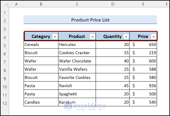
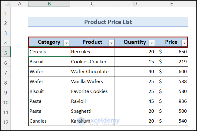
Consider the following data as a product price list. We have added filter to the data. The drop-down icons at the right-bottom corners of the column headers define that the Filter command is added to this range. This enables you to filter the data based on specific criteria within each column.

Why Add Filter in Excel?

Filtering in Excel is a powerful tool that helps analyze data more effectively. Whether you’re working with large datasets or preparing presentations, using filters can help you focus on the most relevant information.

Adding filters in Excel can be beneficial to:

• Manage large datasets;
• Visualize specific data segments;
• Identify and address data inconsistencies;
• Avoid duplicate entries;
• Easy data extraction.

4 Methods to Add Filter in Excel

We will show you how to add filter in Excel from the Data tab, Home tab, and context menu. The keyboard shortcut for adding filter in Excel will be shown as well.

Here are the 4 methods to add filter in Excel:

Adding Filter from Data Tab

The Data tab in Excel provides a dedicated Sort & Filter group with options for sorting and filtering data. The Filter button in this group is used to add or remove filters from the selected range of cells.

To add filter from the Data tab, follow these steps:

1. Select any cell within the range.
2. Go to the Data tab > Sort & Filter group > Filter.
   
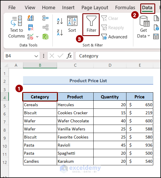   You will see that arrow icons are shown beside the column headers.
   
3. Click the drop-down icon.
4. Select Number Filters > Between.
   The selected column contains numbers. So, the Number Filters option is visible here.
   Thus, Custom Autofilter dialog box will appear.
5. Type the filter criteria > OK.
   Here, we want to filter the values ranging 10-30 in the Quantity column.
   

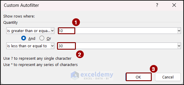
You will see that the Quantity values are shown for only the given range. Here, you will notice that the rows are hidden.

Adding Filter from Home Tab

When you need to do simple filtering tasks without accessing the advanced features available in the Data tab, you can utilize the Filter option from the Home tab.

To add filter from the Home tab, follow the steps:

1. Select any cell within the range.
2. Go to the Home tab > Editing group > Sort & Filter > Filter.
   
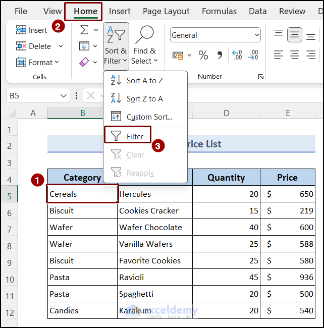
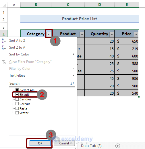
3. Now click on the drop-down icon of your preferred column.
   We have selected the Category column to apply filters.
4. Select the item based on which you want to filter the data.
   You can select multiple items as well.
5. Click the OK button.

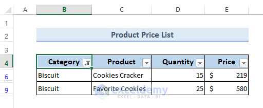
Thus, the data is filtered based on the selected criteria.

Adding Filter from Context Menu

The context menu provides quick access to the Filter command without the need to navigate through the ribbon.

To add filter from the context menu, follow the steps:

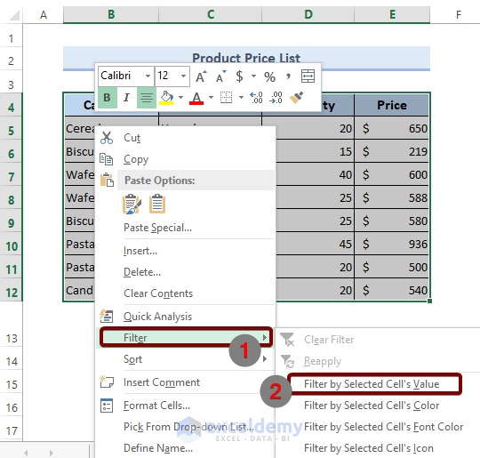
1. Select any cell within the range and right-click on it.
2. Go to Filter > Filter by Selected Cell’s Value.
3. Click on the Filter icon.
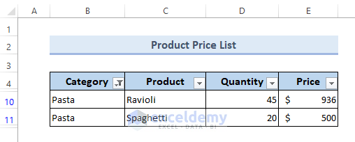
4. Select the item based on which you want to apply the filter.
   Here, we selected the item Pasta from the Category column.
5. Click OK.

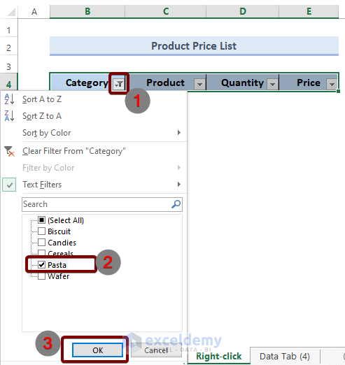
After that, you will see only the products under the Pasta category.

Using Keyboard Shortcut

Using keyboard shortcuts can be a quick and efficient way to perform actions in Excel, especially for tasks that you perform frequently.

To add filter using keyboard shortcut:

1. Select any cell within the range.
2. Press Ctrl+ Shift+ L  and the Filter option will be added to your data.

Now, you can apply filter based on the data in any column.

Download Practice Workbook

Please receive a free copy of the example workbook utilized during the session.

Conclusion

Filtering in Excel helps to focus on specific parts of data, making it easier to analyze and draw insights from large datasets. In this article, we have discussed 4 simple methods of adding filters in Excel. You can apply the method that you find most helpful. We hope this article has helped you solve your problem. If you have questions regarding this topic, please leave a comment.

Frequently Asked Questions

How to filter multiple columns in Excel?

To filter multiple columns in Excel, simply click on the filter arrow for each column you want to filter, and then choose your filtering criteria for each column.

How to remove filter in Excel?

To remove a filter in Excel:

1. Select any cell within the range.
2. Go to the Data tab > Sort & Filter group > Filter.

This will toggle off the filter mode and remove the filter arrows from your data headers.

How to filter blank cells in Excel?

To filter blank cells in Excel:

1. Click on any cell within the range.
2. Go to the Data tab > Sort & Filter group > Filter.
   This will add filter arrows to the headers of your data columns.
3. Click on the filter arrow in the header of the column you want to filter.
4. In the filter drop-down menu, uncheck the Select All option.
5. Scroll down and check the box next to Blanks.

This will filter the column to show only the rows where the selected column is blank.

<< Go Back to Filter in Excel | Learn Excel