Seemanto Saha

Hello Jan,
Thanks for sharing your problem with us. I understand that you want to import data from an authenticated Google Spreadsheet to Excel.

This is a complex method and requires several steps. Since Google Sheets are authenticated using Google Sheets APIs, you have to collect some information like client_id, client_secret, target spreadsheet ID, target spreadsheet name, and the range to be imported.

Here is a step-by-step process:

Step 1: Go to Google Cloud Console and select the target project (i.e. the project used for authenticating the required Google Spreadsheet)

Step 2: Make sure the Google Sheets API is enabled. Navigate the following directory.
APIs & Services >> Library

Step 3: Create an OAuth 2.0 Client ID using the following sub-steps.
Step 3.1: Go to the directory APIs & Services >> Credentials.
Step 3.2: Click the Create credentials button and select OAuth client ID.
Step 3.3: Set the Application type to Desktop App.
Step 3.4: Enter a name for the Application and click the Create button.

This will create a JSON file containing your client ID and client secret. Download the file and open it using VB.net or any other suitable application.

Step 4: Go to the target Excel workbook and open Visual Basic Editor using the keyboard shortcut Alt + F11. Insert a Module and enable the following 3 libraries from Tools >> References directory.

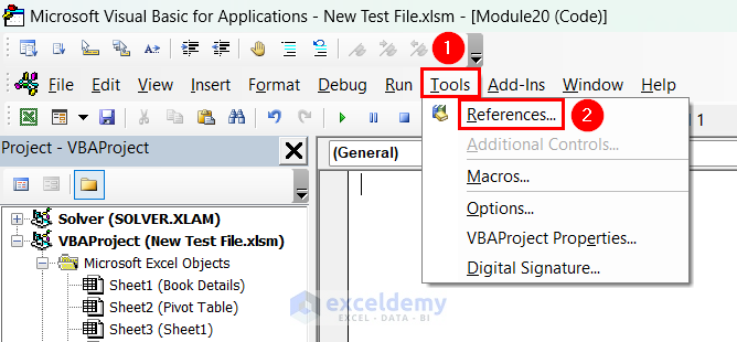
1) Microsoft Scripting Runtime
2) Microsoft XML, v6.0
3) Microsoft VBScript Regular Expressions 5.5

Step 5: Insert the following VBA code and make necessary adjustments (change the spreadsheet ID, client_id, client_secret, sheet name, required range, etc.)

Excel VBA Code

Sub ImportDataFromGoogleSheetToExcel()
    Dim spreadsheetId As String
    Dim rangeName As String
    Dim oAuthApp As Object

    ' Define your Google Sheet details
    spreadsheetId = "1Xz_LyRk0n81VqDjiJYNBMwR1lGSBmm213JtQxK5HRnQ" ' Replace with your Google Sheets document ID
    rangeName = "TestSheet!A1:C10" ' Change to your desired range

    ' Initialize the Google API client
    Set oAuthApp = CreateObject("Scripting.Dictionary")

    ' Configure OAuth2 client
    oAuthApp("client_id") = "304250172616-5ddsaumijhuigr05t8smc1prfqr4m60g.apps.googleusercontent.com"
    oAuthApp("client_secret") = "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"
    oAuthApp("auth_uri") = "https://accounts.google.com/o/oauth2/auth"
    oAuthApp("token_uri") = "https://oauth2.googleapis.com/token"
    oAuthApp("scope") = "https://www.googleapis.com/auth/spreadsheets.readonly"

    ' Wait for the user to authenticate manually (adjust the waiting time as needed)
    Application.Wait Now + TimeValue("00:00:10") ' Wait for 10 seconds

    ' Call the Google Sheets API to get data
    Call ImportDataFromGoogleSheets(oAuthApp, spreadsheetId, rangeName)
End Sub

Sub ImportDataFromGoogleSheets(oAuthApp, spreadsheetId, rangeName)
    ' Create a Google Sheets service instance
    Dim service As Object
    Set service = CreateObject("Scripting.Dictionary")
    service("spreadsheetId") = spreadsheetId
    service("range") = rangeName

    ' Use your OAuth2 client details
    Set service("oauth_client") = oAuthApp

    ' Authenticate with Google Sheets
    Call AuthenticateWithGoogleSheets(service)

    ' Check if the authentication was successful
    If Not service("sheets_service") Is Nothing Then
        ' Fetch data from Google Sheets
        Call GetDataFromGoogleSheets(service)
    End If
End Sub


Sub AuthenticateWithGoogleSheets(service)
    Dim oAuthClient As Object
    Set oAuthClient = CreateObject("MSXML2.ServerXMLHTTP.6.0")

    ' Use your OAuth2 client details
    Dim oAuthApp As Object
    Set oAuthApp = service("oauth_client")

    ' Authenticate with Google Sheets using OAuth2
    Dim authUrl As String
    authUrl = oAuthApp("auth_uri") & "?client_id=" & oAuthApp("client_id") & "&redirect_uri=urn:ietf:wg:oauth:2.0:oob&scope=" & oAuthApp("scope") & "&response_type=code"
    Call OpenDefaultBrowser(authUrl)

    ' Wait for the user to authenticate manually
    Application.Wait Now + TimeValue("00:00:10") ' Wait for 10 seconds

    ' Check if the user is authenticated
    Dim authCode As String
    authCode = InputBox("Enter the authorization code: ")

    ' Exchange the authorization code for an access token
    Dim postData As String
    postData = "code=" & authCode & "&client_id=" & oAuthApp("client_id") & "&client_secret=" & oAuthApp("client_secret") & "&redirect_uri=urn:ietf:wg:oauth:2.0:oob&grant_type=authorization_code"

    oAuthClient.Open "POST", oAuthApp("token_uri"), False
    oAuthClient.setRequestHeader "Content-Type", "application/x-www-form-urlencoded"
    oAuthClient.send postData

    Dim responseText As String
    responseText = oAuthClient.responseText
    Dim accessToken As String
    accessToken = GetJsonValue(responseText, "access_token")

    ' Create a service to interact with Google Sheets
    Dim sheetsService As Object
    Set sheetsService = CreateObject("MSXML2.ServerXMLHTTP.6.0")
    sheetsService.Open "GET", "https://sheets.googleapis.com/v4/spreadsheets/" & service("spreadsheetId") & "/values/" & service("range"), False
    sheetsService.setRequestHeader "Authorization", "Bearer " & accessToken

    ' Check if authentication was successful
    If sheetsService.Status = 200 Then
        Set service("sheets_service") = sheetsService
    Else
        MsgBox "Authentication failed. Please try again."
    End If
End Sub

Sub GetDataFromGoogleSheets(service)
    Dim sheetsService As Object
    Set sheetsService = service("sheets_service")

    ' Send a request to get data from Google Sheets
    sheetsService.send

    ' Check if the request was successful
    If sheetsService.Status = 200 Then
        Dim responseText As String
        responseText = sheetsService.responseText

        ' Parse the response data (you can customize this part)
        Dim data As Variant
        data = ParseGoogleSheetsData(responseText)

        ' Paste the data into the active sheet starting from cell A1
        Dim targetSheet As Object
        Set targetSheet = ThisWorkbook.Sheets(1) ' Change to your target sheet
        targetSheet.range("A1").Resize(UBound(data, 1), UBound(data, 2)).Value = data
    Else
        MsgBox "Failed to retrieve data from Google Sheets."
    End If
End Sub

Function GetJsonValue(jsonString As String, key As String) As String
    ' A function to extract a value from a JSON string given a key
    Dim regex As Object
    Set regex = CreateObject("VBScript.RegExp")

    regex.Global = True
    regex.MultiLine = False
    regex.IgnoreCase = True
    regex.Pattern = """" & key & """:\s*""(.*?)"""

    If regex.Test(jsonString) Then
        GetJsonValue = regex.Execute(jsonString)(0).SubMatches(0)
    Else
        GetJsonValue = ""
    End If
End Function

Function ParseGoogleSheetsData(data As String) As Variant
    ' A function to parse Google Sheets data from JSON to a 2D array
    Dim json As Object
    Set json = JsonConverter.ParseJson(data)

    Dim values As Object
    Set values = json("values")

    Dim numRows As Long
    numRows = values.Count

    Dim numCols As Long
    numCols = values(1).Count

    Dim resultArray As Variant
    ReDim resultArray(1 To numRows, 1 To numCols)

    Dim i As Long, j As Long
    For i = 1 To numRows
        For j = 1 To numCols
            resultArray(i, j) = values(i - 1)(j - 1)
        Next j
    Next i

    ParseGoogleSheetsData = resultArray
End Function

Step 6: Run the code and the required data from the authenticated Google Sheets will appear in your Excel Active Sheet.

Note that, this code will only work if you have the Google Sheets API developers have authorized your email to the target Google Spreadsheet.

Hopefully, we were able to help you. Let us know your feedback.

Regards,
Seemanto Saha
ExcelDemy

Dear AHMET KARAASLAN,
Thanks for your comment.

Although the mentioned formula is an array formula, you can use it in Excel for Microsoft 365 without any modifications.

Enter the formula in your required cell and press the Enter key. After that drag down the Fill Handle icon.

Note: This formula can return #NUM! error if any match isn’t found when you use the Fill Handle feature. To avoid this you can combine the IFERROR function with your formula. The modifier formula is:

=IFERROR(INDEX($C$5:$C$11, SMALL(IF(ISNUMBER(MATCH($B$5:$B$11, $B$14, 0)), MATCH(ROW($B$5:$B$11), ROW($B$5:$B$11)),””), ROWS($A$1:A9))),””)

However, if you want to avoid using the Fill Handle feature and want all match results with a single formula, then you can use the FILTER function. This function is only available in Excel for Microsoft 365 and can filter a range based on any given criteria.

To get the same result as the INDEX-MATCH method, apply the following formula in the required cell and press the Enter key.

=FILTER(C5:C11,B5:B11=B14)

I hope this solution will be helpful for you. Let us know your feedback.

Regards,
Seemanto Saha
ExcelDemy

Hello JOHN C,

Yes, you are right, the formula for calculating the Mix value is different in the given Excel file and the above article.

The formula mentioned in our article is correct. There must have been an error while selecting cell E11, hence the adjacent cell D11 is present in the Excel file formula.

We have updated the Excel file with the correct formula. Thanks for your feedback.

Regards,
Seemanto Saha
Exceldemy

Dear Agnes,

To obtain similar results in Google Sheets, we have to create a similar dataset, click on the Extensions menu, and select Apps Script from the options.

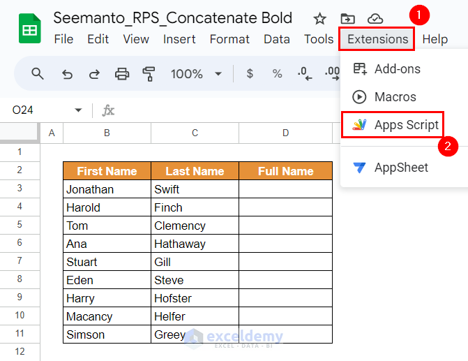
Then in the new window, we have to replace the default script with the following script:

function boldTextInConcatenate() {
  var ss = SpreadsheetApp.getActiveSpreadsheet()
  .getSheetByName("Bold in Concatenate");
 
  var lastRow = ss.getLastRow();


  var bold = SpreadsheetApp.newTextStyle()
  .setBold(true)
  .build();


  for (var i=3;i<=lastRow;i++){
    var fName = ss.getRange(i,2).getValue();
    var lName = ss.getRange(i,3).getValue();
   
    var richText = SpreadsheetApp.newRichTextValue()
    .setText(fName+' '+lName)
    .setTextStyle(0, fName.length, bold)
    .build();
   
    ss.getRange(i,4).setRichTextValue(richText);
  }
}

Afterward, we have to Save and Run the script. The output should be like the following:

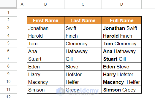
You can download the Spreadsheet from the link below:
Bold text in Concatenate

Let us know your feedback.

Regards,
Seemanto Saha
ExcelDemy