How to Apply a Bottom Double Border in Excel – 2 Methods

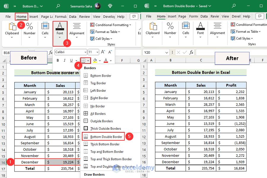
In the following image, the Bottom Double Border is applied in the row before the Total row using the built-in Border option in the Font tab.

Method 1 – Using the Built-in Border Option

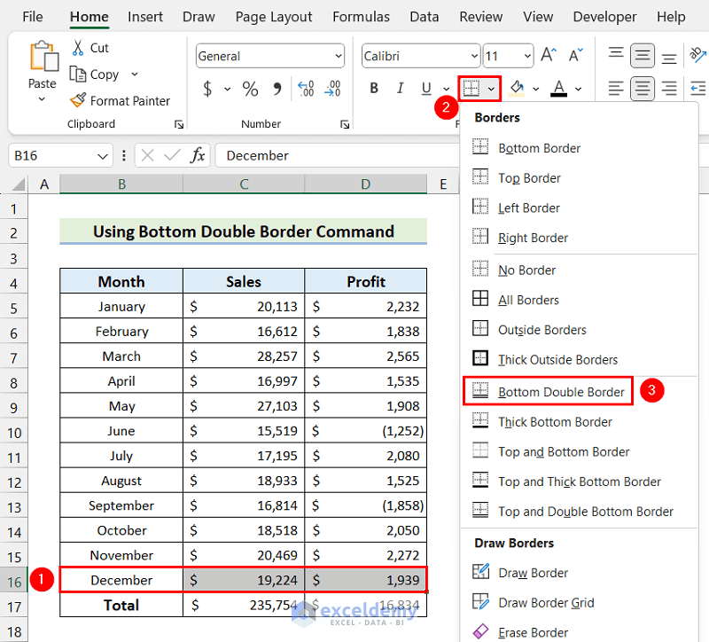
• Select the range. Here, B16:D16.
• Go to the Home tab > Font > Border > Bottom Double Border.

Tip: To apply a Line Color or Line Style other than default, choose it in Line Color and/or Line Style in Draw Borders first, and then select the borders.

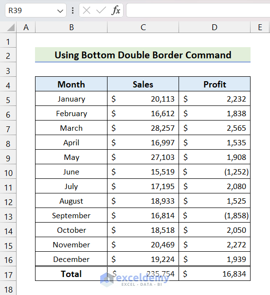
This is the output.

Note: You can also apply the Bottom Double Border using a shortcut: Select the range and press Alt + H + B + B one by one.

Read More: How to Insert Border in Excel

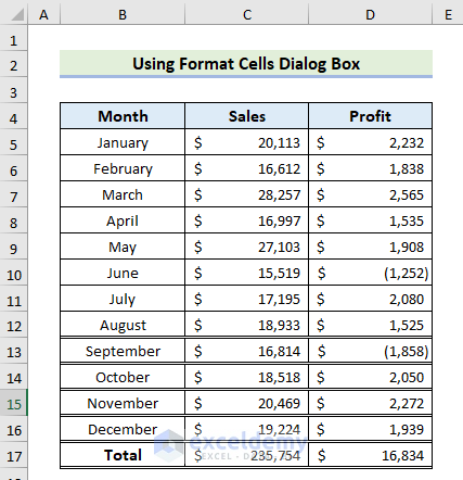
Method 2 – Using the Format Cells Dialog Box

• Select the range. Here, B12:D17.
• Right-click and click Format Cells.
  You can also click the Format Cells dialog box launcher icon in Font, Number, or Alignment.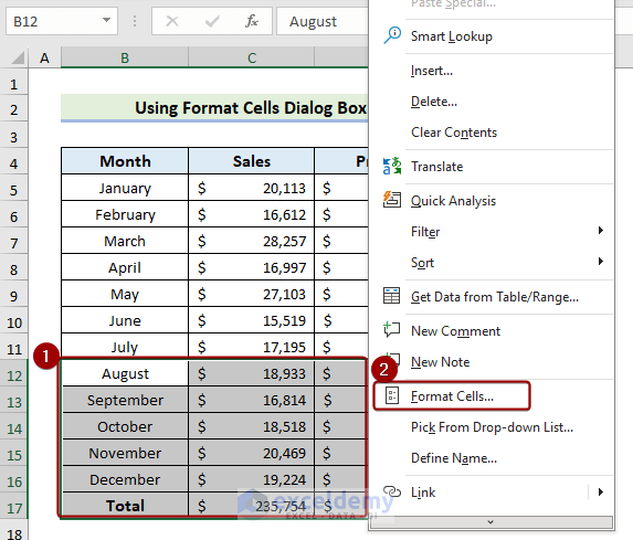
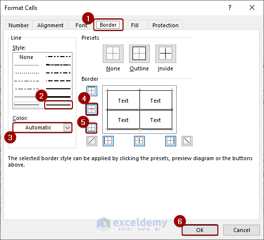
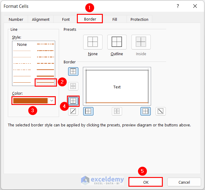
• In the Format Cells dialog box:
  • Go to the Border tab.
  • Select Double Border.
  • Choose a color in Color.
  • Select the middle and bottom border in Border.
  • Click OK.

  

The selected range has a Double Bottom Border:

Note: You can press Ctrl+1 to open the Format Cells dialog box.

Read More: How to Apply All Borders in Excel

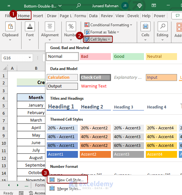
How to Create a Custom Bottom Double Border Style in Excel

• Go to the Home tab > Cell Styles > New Cell Style.
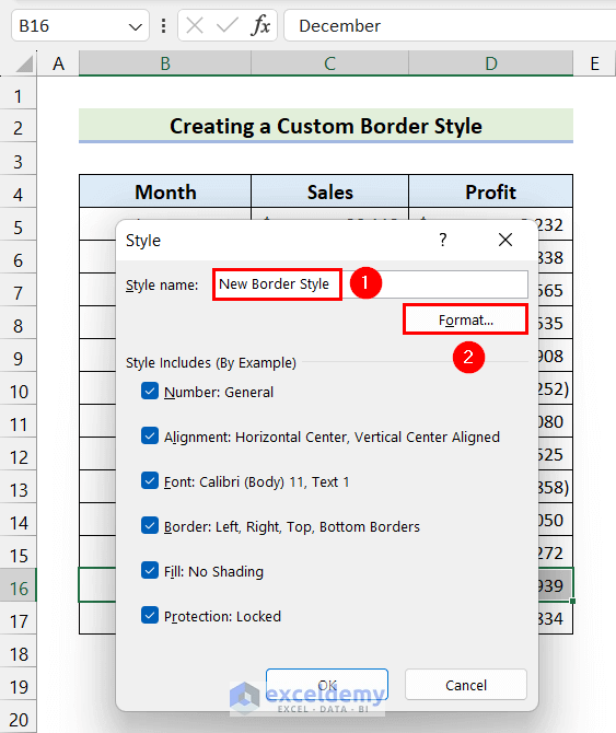
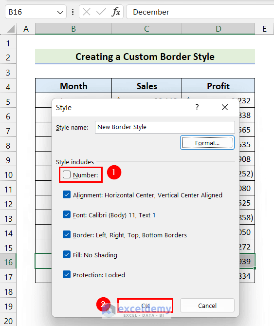
• In the Style dialog box, set a Style Name and click Format.
• In the Format Cells dialog box:
  • Go to the Border tab.
  • Select Double Border.
  • Choose a Color.
  • Select Bottom Border.
  • Click OK.

  

• Uncheck Number and click OK.
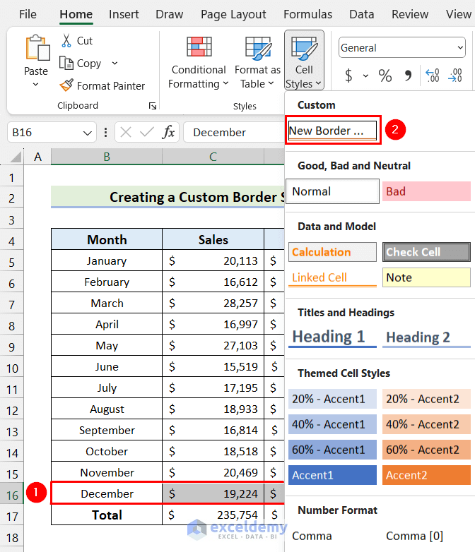
• Select the range. Here, B16:D16.
• Click  Cell Styles and select the created custom cell style.

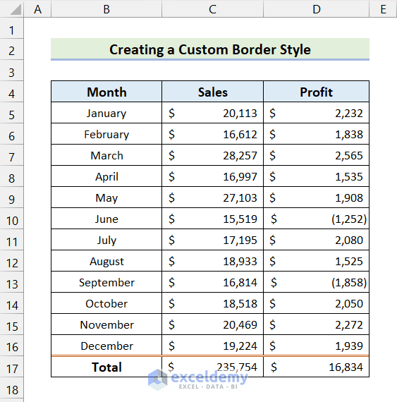
The custom border style will be applied to the selected range:

Read More: How to Add Thick Box Border in Excel

Frequently Asked Questions

How to Remove a Double Bottom Border in Excel?

To remove a Double Bottom Border from a range of cells: select the range > click Borders > select No Border. You can also press Ctrl + Shift + _ to remove all borders.

Is the Double Underline Feature the same as the Double Bottom Border in Excel?

The Double Underline feature is usually applied to the content of a cell and the Double Bottom Border to the cell itself.

To apply the Double Underline feature: select the cell > click Underline > select Double Underline.

Download Practice Workbook

Download the following workbook and practice.

Related Articles

• How to Add or Remove Dotted Border in Excel
• How to Add Cell Borders Inside and Outside in Excel
• How to Remove Borders in Excel
• How to Apply Top and Bottom Border in Excel

<< Go Back to Cell Borders in Excel | Excel Cell Format | Learn Excel