How to Lock Borders in Excel (With Easy Steps)

In this article, we will explain how to lock the borders of a table in a few easy steps.

Step 1 – Creating a Dataset

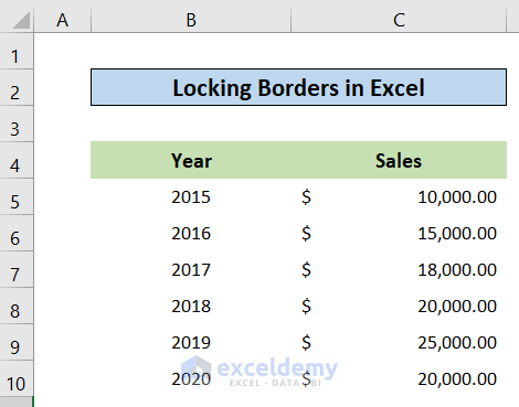
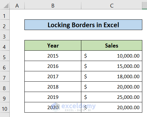
To start with, we need a table whose borders we can lock. We’ll use the dataset below, which has no borders.

Read More: How to Insert Border in Excel

Step 2 – Open Conditional Formatting

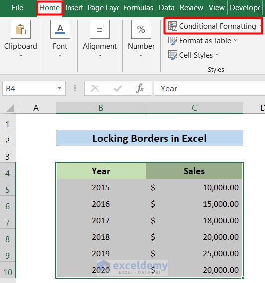
We’ll apply conditional formatting to lock the table borders.

• Select the whole dataset.
• Go to the Home tab on the ribbon
• Select Conditional Formatting.

Step 3 – Apply a New Rule

We’ll now apply a new conditional formatting rule to lock the borders.

• From the Conditional Formatting drop-down, select New Rule.

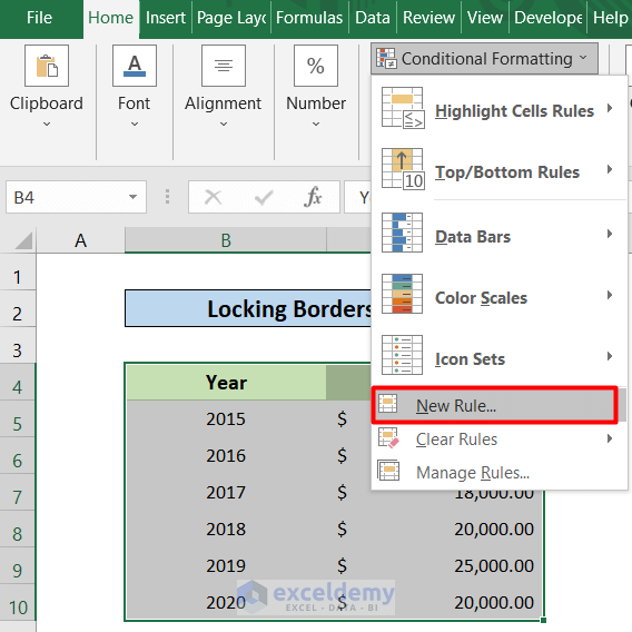
• The New Formatting Rule window will pop up.
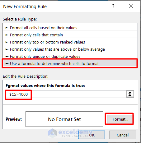
• Select the option indicated in the picture below.
• Enter the following formula in the indicated box:

• Click Format.

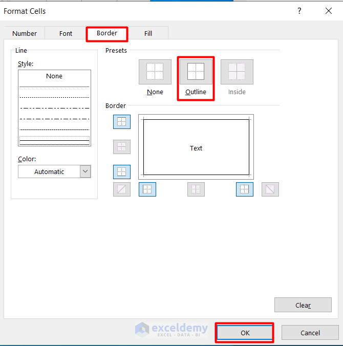
The Format Cells dialog box opens

• Select the Border tab.
• Select the Outline option.
• Click OK.

Read More: How to Change Border Color in Excel

Step 4 – Show the Final Result

As result of the preceding steps, the result looks just like the picture below.

Read More: How to Cancel Moving Border in Excel

Download the Workbook

Related Articles

• How to Make Graph Paper in Excel
• How to Remove Page Border in Excel
• [Fixed!] Border Not Showing in Excel

<< Go Back to Cell Borders in Excel | Excel Cell Format | Learn Excel