How to Insert Border in Excel (3 Effective Methods)

Inserting borders in Excel refers to the process of adding lines or boundaries around cells, ranges, or tables to enhance the visual appearance of the data. You can also highlight important details, create clear sections, or enhance readability in a spreadsheet by doing this.

In this Excel tutorial, you will learn to insert borders.

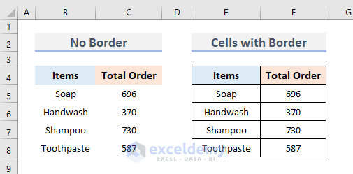
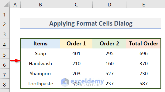
Here, on the left of the image, cells have no borders, while on the right, cells are bordered.

3 Methods to Insert Border in Excel

You will learn to insert border in 3 ways using the Excel Ribbon, Format Cells dialog box, and the Draw Border option.

Using Excel Built-in Borders Option

To insert border, use the built-in Border option in the Font group of Excel Ribbon. Follow the steps below:

1. Select the range of data.
2. Go to the Home tab > Font group > Border drop-down.
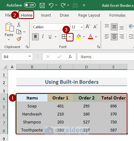
3. Select any of the border options from the dropdown.
   For example, you may apply the All Borders option.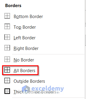

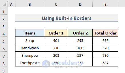
You will find the following output in your worksheet after applying the border.

Note: To insert an outside border easily: select the set of data and press Ctrl + Shift + & from the keyboard.

Read More: How to Remove Borders in Excel

Using Format Cells Dialog

If you use the Excel Ribbon to insert borders, you will get some fixed type of border list. But in the Format Cells dialog box, you will get additional options for inserting borders, like different colors and designs.

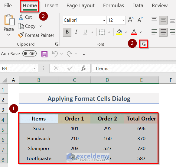
To insert border using Format Cells dialog box, follow the steps:

1. Select the set of data.
2. Go to Home tab > Font group > Font Settings dialog box launcher.Format Cells dialog box will pop up. You can also press Ctrl+1 together to open the dialog box.
3. In the Format Cells dialog box:
   • Go to the Border tab.
   • Choose the line style and color from the Style and Color option.
   • Choose a Presets option.
     Or, apply borders individually from the Borders section.
   • Click OK.

   

You will see the following output in your worksheet.

To add borders quickly, you can apply some shortcuts in the Format Cells dialog box:

• For the Left Border, type: Alt + L
• For Right Border, type: Alt + R
• For Top Border, type: Alt + T
• For the Bottom Border, type: Alt + B
• For the Upward diagonal, type: Alt + D
• For Horizontal interior, type: Alt + H
• For Vertical interior, type: Alt + V

Read More: How to Apply Bottom Double Border in Excel

Using Draw Border

You can draw borders directly on the worksheet rather than selecting cells first and then selecting from built-in options. This method is useful when you want to apply a border to non-adjacent cells. However, using this method for a large set of data is time-consuming.

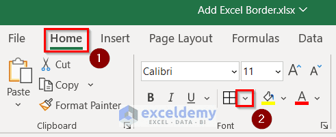
To draw border in a cell, follow the steps below:

1. Go to the Home tab > Font group > Border drop-down.
2. Select Draw Border from the drop-down.
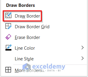
   Excel switches to the Draw Border mode automatically, and the cursor becomes a pen.
3. Take the mouse pointer to the cell where to apply the border.
4. Click on the side of the cells where you want to apply the borders.
5. If done, press Esc to disable the border pen.

From the gif below, you will understand the process of applying Draw Border option to insert border in Excel.

Note: You can use the Draw Border Grid option to apply border to the whole set of data. Select the Draw Border Grid from the Borders drop-down option and drag the pen on your desired data range. The following gif is for better understanding:

How to Insert Custom Border Style in Excel

Using built-in border style or Format Cells dialog box for multiple cells is time-consuming. A better alternative is to create a custom border style and use it while working.

To create a customized border style, follow the steps below:

Step 1: Create New Style and Name It

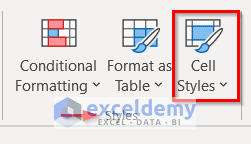
1. Go to the Home tab > Styles group > Cell Styles.
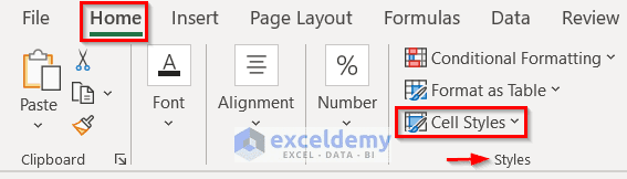
2. Click on New Cell Style from the drop-down menu.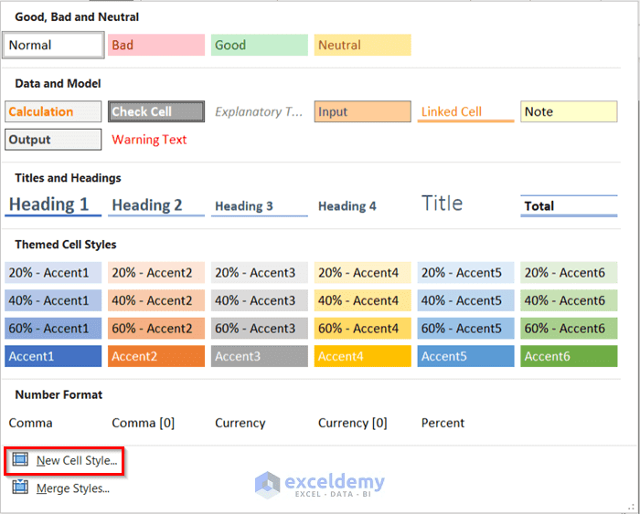A dialog box naming Style will pop up.
3. In the Style dialog box:
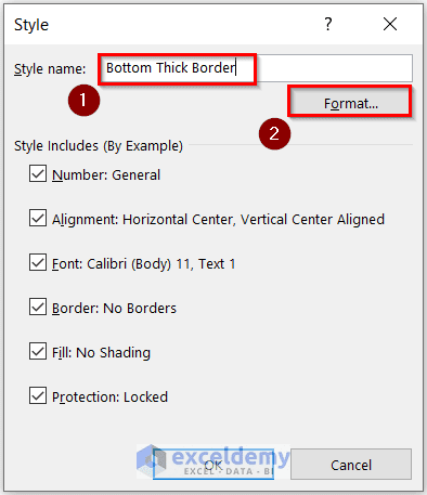
   • Type a border style name of your own choice in the Style name box.
   • Click on Format.
4. The Format Cells dialog box is now open.

Step 2: Format the Newly Created Style

1. In the Format Cells dialog box:
   • Go to Border tab.
   • Select any line Style and Color from the Line group.
   • Choose any border option from the Border.
   • Click OK.

   

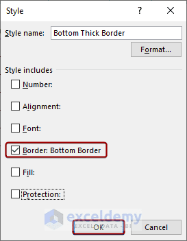
2. Again, from the Style window, check the box Border: Bottom Border.
3. Click OK.

Our new customized style is ready to use.

Step 3: Apply the Customized Border

1. Select the cells.
2. Go to the Home tab.
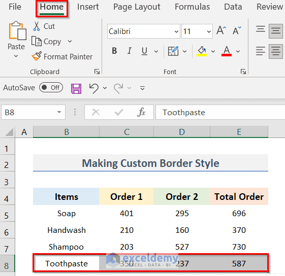
3. Click on Cell Styles in the Styles group.A drop-down menu will appear.
4. Select the newly created custom border style from the Custom group.
   

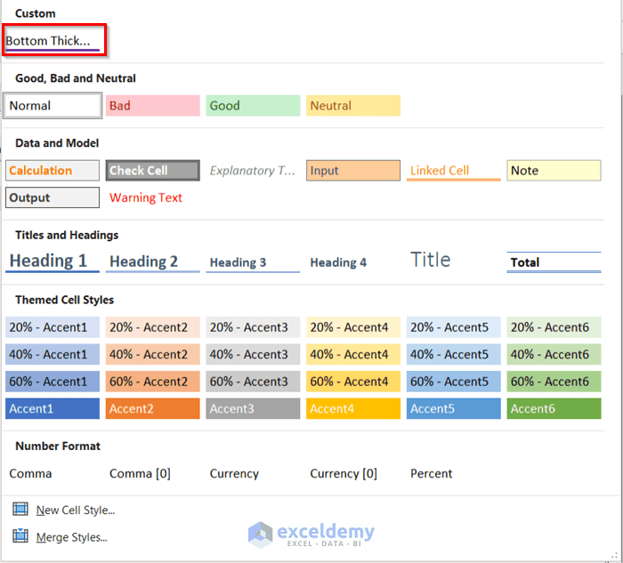
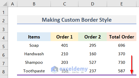
You will find that the new border style is applied to the selected cells.

Read More: How to Change Border Color in Excel

Download Practice Workbook

Download the practice workbook from here.

Conclusion

This is the end of the article on inserting border in Excel. We have discussed the 3 different methods of inserting border in Excel. We have also covered how to create custom border in Excel. Use the method which perfectly matches your criteria. If you find any other method to insert border in Excel, please let us know. Comment if you face any trouble while working. Thank you!

Frequently Asked Questions

How to copy borders from one cell to another?

Select the cell with the desired border. Press Ctrl + C to copy. Then select the target cell and press Ctrl + Alt + V to open the Paste Special menu. Choose “Formats” to copy the border.

How to add a double border to cells in Excel?

Go to “Borders,” choose “More Borders,” and select the “Double” option.

How to remove border in Excel?

To remove border in Excel, use the built-in Border option. Just select the No Border option from the drop-down.

Related Articles

• How to Add Thick Box Border in Excel
  
• How to Add or Remove Dotted Border in Excel
• How to Add Cell Borders Inside and Outside in Excel
  
• How to Apply Top and Bottom Border in Excel

<< Go Back to Cell Borders in Excel | Excel Cell Format | Learn Excel