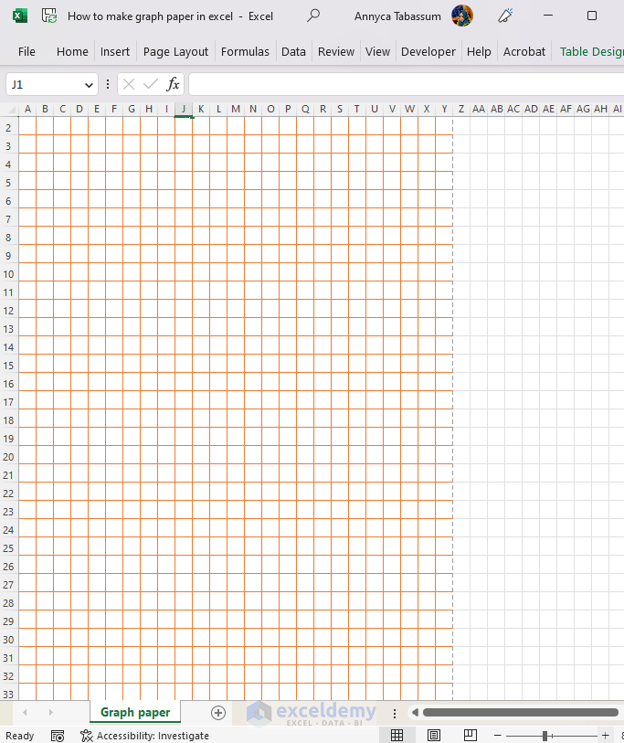
In this tutorial, we will guide you through the step-by-step process of how to make graph paper in Excel. Microsoft Excel provides the flexibility to create graph paper according to your specific needs. Excel’s grid structure and formatting capabilities make it an ideal tool for generating precise and professional-looking graph paper.
How to Make Graph Paper in Excel: Step-by-Step Procedures
In Excel, while you are making a graph paper, it allows you to generate custom layouts, adjust grid spacing, and incorporate additional features to suit your requirements. To generate a professional-look graph paper you have to follow the steps below:
Step 1: Change Page Layout and Margin
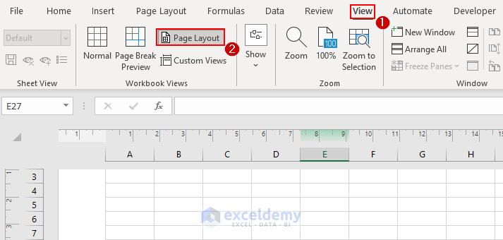
To make this process easier, first, you have to convert the page into the Page Layout view. Because Excel cells are measured in points in other page views, but in Page Layout view, you can resize cells using standard measurement. To convert the page view, follow the steps below:
- First, go to the View tab, and from the Workbook Views group choose the Page Layout view.
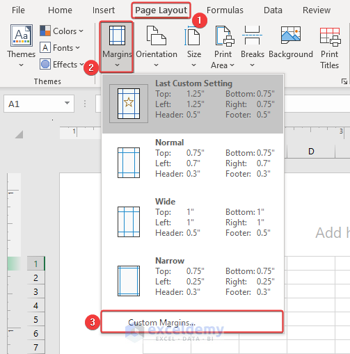
- To make the graph more presentable, change the margin width to 1.25 inches from all sides.
- To make it happen, go to the Page Layout >> Margins >> Custom Margins option.
- Go to the Margins tab and set the Top, Bottom, Left, and Right margins to 1.25 inches.
- Set the Header and Footer to 0.5 inches.
- Also, check Horizontally and Vertically under Center on page and click on OK.
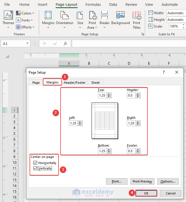
Note: You can set the value of the margin as per your requirement
Step 2: Insert a Table
To provide grids for the graph, in this step, you have to insert a table by selecting a desired portion of cells. To add a table,
- Go to the Insert >> Table option and insert a table.
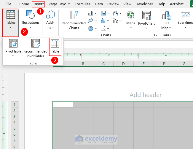
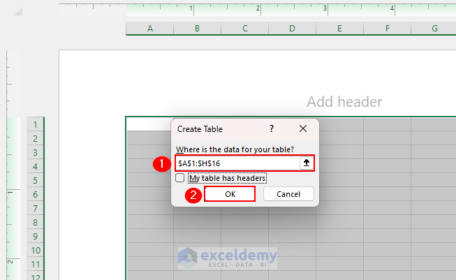
- Select a range of cells and click on OK.
- Alternatively, Use the keyboard shortcut Ctrl + T to insert a table and select a portion of the sheet to create a table to develop grids for the graph.
- While the table comes up, you will find a new tab Table Design added in the ribbon.
- In the Table Design tab, some table style is checked by default.
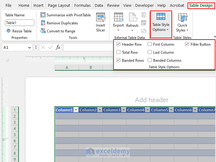
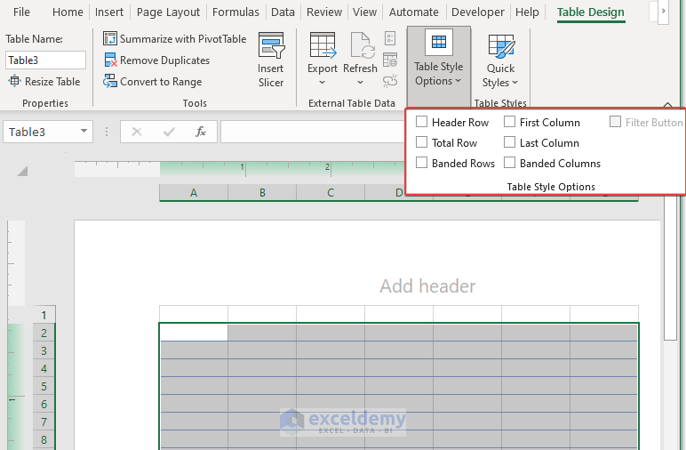
- Uncheck all the selections.
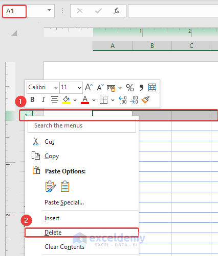
At the end of this step delete the top row to make the resizing process easier.
- Select the top row and right-click on it.
- Choose Delete from the list.
Step 3: Resize Column Width and Row Height
Now it’s time to resize the column width and row height to create a graph paper. You have to bear in mind that resize the columns and rows after inserting the table otherwise you have to resize them again.
- To change the column width, select all the cells by clicking on the triangle symbol in the top left corner. Or you can apply the keyboard shortcut Ctrl + A.
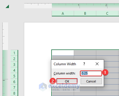
- Keep the cursor on the column section.
- Simply right-click and choose the Column Width option from the Context Menu.

- We change the column width to 0.25 inches and click on OK.
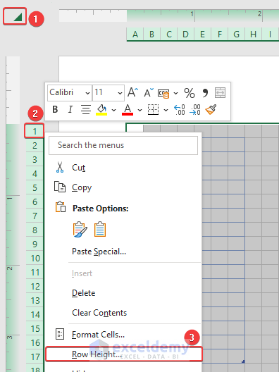
- Similarly, select all the cells and move the cursor to the left of the sheet on the row number, and right-click on it.
- Select the Row Height option.
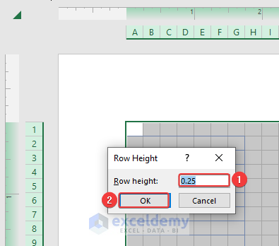
- Change the row height to 0.25 inches, the same as the column width. You can select different values as per your requirements.
Step 4: Customize Table to Fit the Page
In this step, you have to customize the table to fit with the page and can also modify the color to make it more visible. To do so,
- You will find a triangle in the bottom right corner of the table.
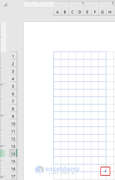
- Select it and simply drag the area you want to fit on a page.
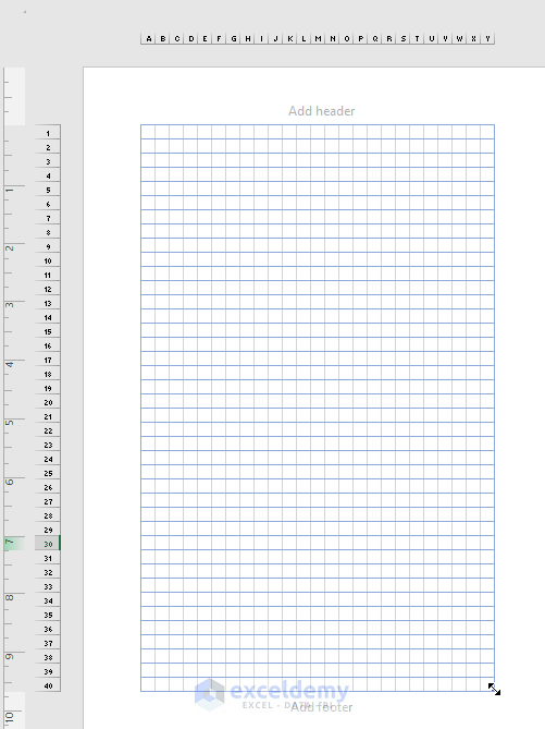
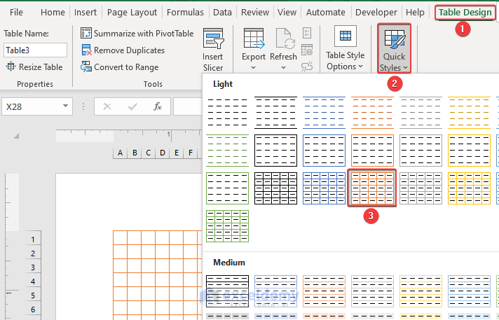
- To make the graph more visible, you can add color by using the Table Design bar.
- Go to the Table Design bar, expand the Quick Style option, and select a design that you want.
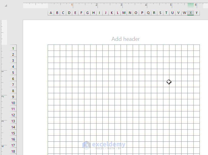
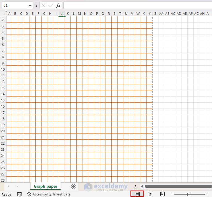
- Now you will get the customized table.
- Finally, go back to the Normal view of the worksheet.
Step 5: Save the Changes
If you want to reuse your custom graph paper, you need to save it and use it whenever necessary. To save the graph as an Excel workbook,
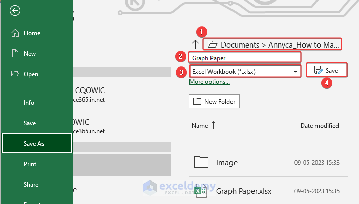
- Go to the File >> Save As option.
- After that, chose a location in the computer to save the file, we selected the Document folder to save
- Provide a name for the template, we name it “Graph Paper”. And specify the file type (.xlsx).
- Click Save to store the template for further use.
Read More: How to Change Border Color in Excel
How to Print the Graph Paper in Excel
If you want a hard copy of the customized graph paper in Excel, you can easily get that by using the Print option. To print out the graph,
- Go to the File tab and select the Print option.
- Then, check the print settings to ensure they match your requirements.
- Click on Print to get the hard copy.
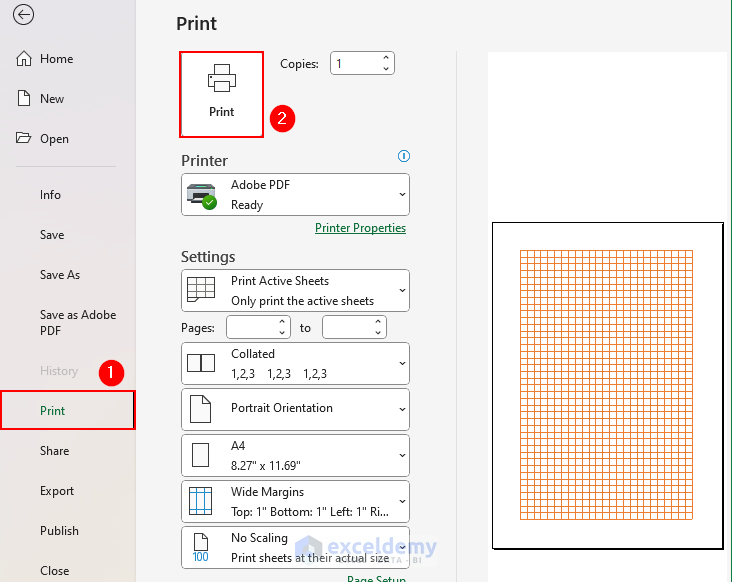 You will get Print Preview on the right side of the image.
Read More: How to Remove Page Border in Excel
Use of Graph Paper in Excel
Excel’s graph paper-like grid offers a versatile platform for a wide range of applications, from artistic endeavors to data analysis and planning. Its flexibility and computational capabilities make it a powerful tool for both professional and personal use. The utilizing field of graph paper in Excel includes:
- Excel’s grid-like structure of graph paper makes it suitable for creating drawings or sketches.
- Graph paper in Excel provides a convenient framework for organizing and visualizing data. You can use the cells as data points and create graphs or charts within the grid to represent data in a visual format.
- Excel’s graph paper-like grid can be used for performing mathematical calculations, plotting graphs, or conducting scientific experiments. You can input equations or formulas into cells and utilize Excel’s built-in functions to perform calculations and generate results.
- The grid layout of Excel is ideal for creating schedules, calendars, or project plans. You can use the cells to allocate time slots, assign tasks, or track progress. By adjusting the size of cells, you can create a customized layout that suits your planning needs.
- Excel’s graph paper can be used as an educational tool for teaching various subjects such as mathematics, physics, or computer science. It provides a structured environment for demonstrating concepts, solving problems, or conducting simulations.
Frequently Asked Questions
1. Is it possible to customize the spacing between the squares on the graph paper in Excel?
Yes, it is possible to customize the spacing between squares on graph paper in Excel by adjusting the row height and column width. By setting them to specific values, you can create a grid with evenly spaced squares.
To achieve this, you need to determine the size of each square and then adjust the row height and column width accordingly. To do so,
- Open Excel and create a new workbook or open an existing one.
- Select the cells that you want to adjust the size for. If you want to adjust the entire worksheet, you can click on the triangle button at the intersection of row numbers and column letters (top-left corner of the sheet) to select all cells.
- Right-click on any of the selected cells and choose Row Height or Column Width from the context menu.
- In the Row Height or Column Width dialog box, you can specify the desired size.
By setting the row height and column width to the desired values, you can customize the spacing between squares on the graph paper in Excel.
2. How can I remove the gridlines from the graph paper in Excel?
To remove the gridlines from the graph paper in Excel, you can follow these steps:
- Open Excel and open the workbook containing the graph paper or create a new workbook.
- Select the cells or range of cells that you want to remove the gridlines from. If you want to remove gridlines from the entire worksheet, you can click the triangle button at the intersection of row numbers and column letters to select all cells.
- Go to the View tab on the Excel ribbon and uncheck the Gridline option.
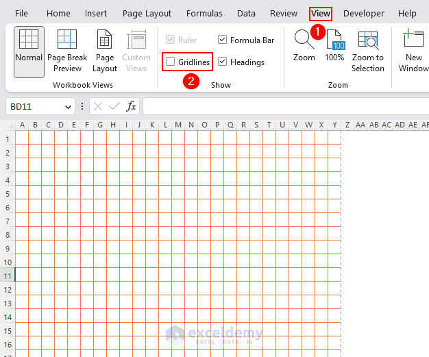
The gridlines will be removed from the selected cells or the entire worksheet if you had selected all cells. The graph paper in Excel will appear without any visible gridlines.
3. Can I print multiple pages of the graph paper in Excel?
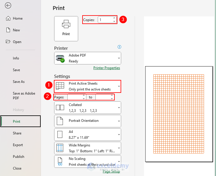
Yes, you can print multiple pages of the graph paper in Excel. Excel provides various printing options that allow you to control the number of pages and the layout of the printed graph paper. To print multiple pages,
- Make sure the Print Active Sheets or Print Entire Workbook option is selected, depending on whether you selected specific cells or the entire worksheet.
- If you want to print a specific range of pages, you can enter the desired page range in the Pages field. For example, you can enter 1-5 to print the first five pages.
- If you want to print a single page multiple times, you can select the Copies option from the Print menu and add the number of copies you desire.
Things to Remember
- You have to insert the table first, then resize the columns and rows.
- Insert the same column width and row height to get perfect square grids.
- Before printing, the worksheet must be on Page Layout view.
You can download this practice workbook while going through this article.
Conclusion
We believe after completing the article, you will develop a proper knowledge of how to make graph paper in Excel. Moreover, you can also learn how to save and print hard copies of graph paper and use graph paper as well. For further queries, you can comment below. Goodbye!
Related Articles
- How to Lock Borders in Excel
- [Fixed!] Border Not Showing in Excel
- How to Cancel Moving Border in Excel
<< Go Back to Cell Borders in Excel | Excel Cell Format | Learn Excel
Get FREE Advanced Excel Exercises with Solutions!
