Worksheet Formatting (Ultimate Guide)

Worksheet formatting in Excel involves changing the font style, fill color, border style, adjusting row height, column width, number formats, etc. of a sheet. Worksheet formatting is often required to increase the readability of data.

In this Excel tutorial, you will learn about the necessary features to format a worksheet. We will start our process with an unformatted worksheet and use various Excel features to format the worksheet.

The following image shows an overview of formatting a worksheet to increase readability and effectively visualize the data.

What Is the Importance of Worksheet Formatting in Excel?

Formatting a worksheet isn’t about the aesthetic only. It enhances readability, helps in data interpretation, and showcases professionalism. Finding required data from a properly formatted worksheet is easier compared to a messy worksheet. Formatting the worksheet also facilitates effective data analysis from the worksheet.

11 Examples of Formatting Worksheet in Excel

To format a worksheet, you need to change cell shading, borders, fonts, data alignment, and various other elements of a worksheet. Consider the following dataset in an Excel worksheet. There is a data table in range B4:G15 and a title in Cell B2. The data table contains the Brand, Device, Model, Origin  Country, Release Date, and Price of various technological products.

The worksheet is not formatted yet, so the dataset is poorly visualized and difficult to understand. To fix this problem, we will format the worksheet using various Excel features.

Here are 11 examples of formatting a worksheet in Excel:

1. Turning Off Gridline in an Excel Worksheet

In this section, we will turn off the gridlines. Apply the following steps for that:

1. Go to the View tab.
2. Uncheck the Gridlines option to disable it.

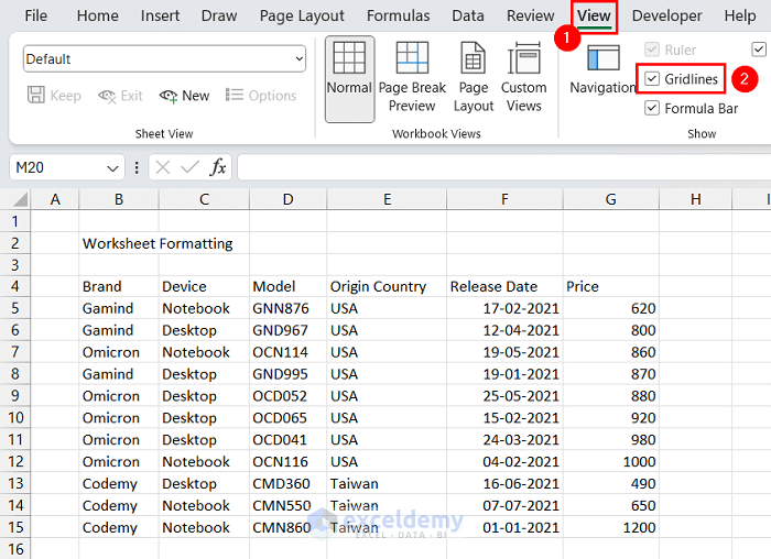
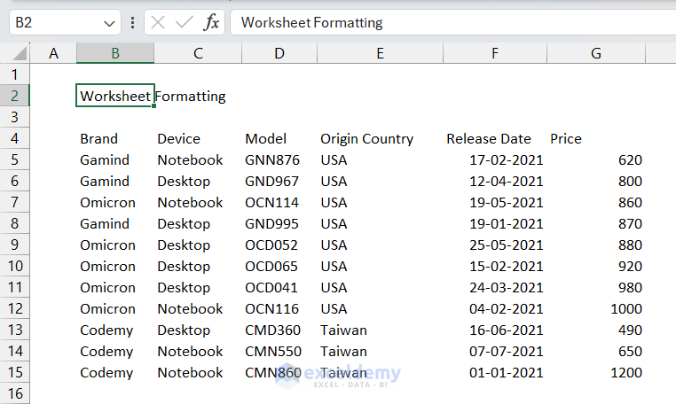
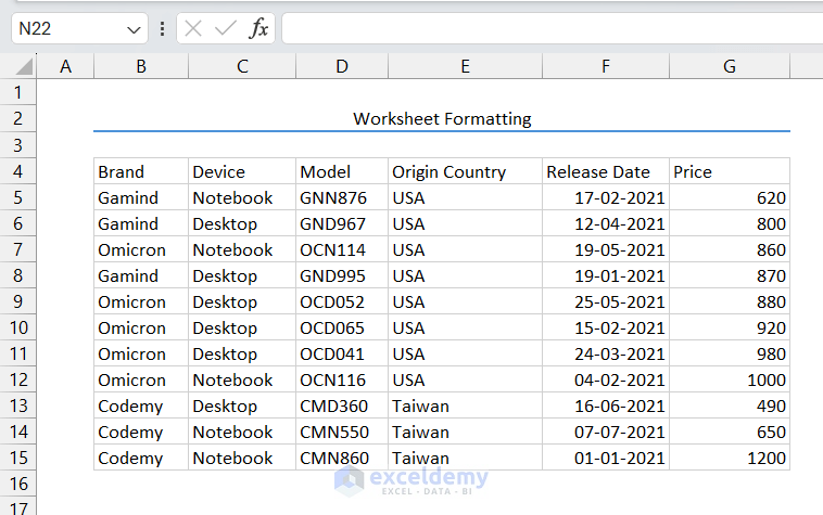
As a result, the gridlines will turn off from the worksheet.

2. Formatting Title in Excel Worksheet

In this section, we will format the title. Instead of displaying the title in one corner of the row, we want the title in the center of the row.

Here are two ways to do this:

2.1 Using Merge & Center Command

You can use the Merge & Center command to merge the cells of the above data table in the row of the title. This command will align the data in the center of the merged cells.

To apply the Merge & Center feature to format the title, apply the following steps:

1. Select the row of the title.
   Here, I have selected the range B2:G2.
2. Go to Home tab > Alignment group > Merge & Center command.

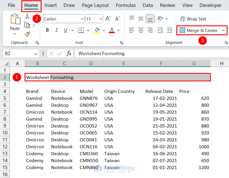
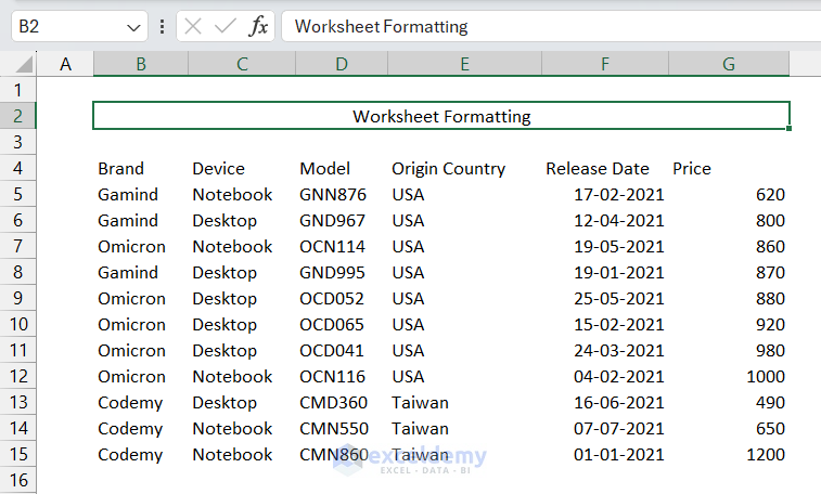
This will merge all the selected cells and bring the title to the center of the merged cell.

2.2 Using Center Across Selection Option

Merging cells often creates problems in formula-based operations in Excel. To avoid such issues, you can use the Center Across Selection option as an alternative. This option only displays the value as center-aligned. But the value is stored in a single cell only.

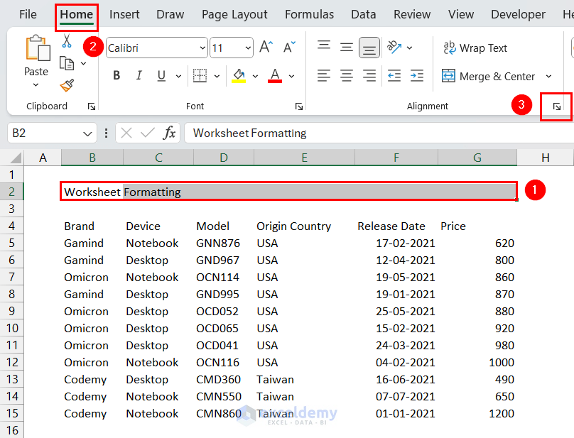
To format the title with the Center Across Selection option, follow the steps below:

1. Select the row of the title.
   Here, I have selected the range B2:G2.
2. Click the Format Cells dialog box launcher from the Alignment group.
   
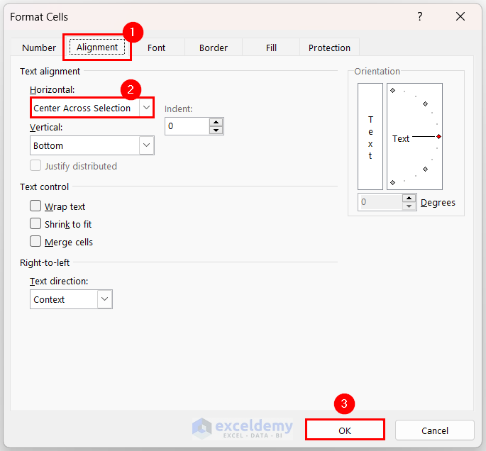
   As a result, the Format Cells dialog box will appear.
3. In the Format Cells dialog box:
   • Go to the Alignment tab.
   • Set the Horizontal Text Alignment to the Center Across Selection option.
   • Click OK.

   

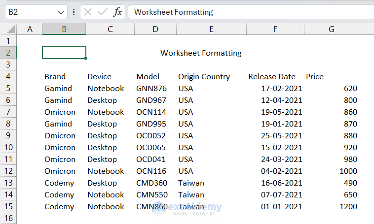
This will display the title center-aligned to the row. However, you can notice that the title value is in a single cell (cell B2 in this case).

3. Applying Cell Borders in an Excel Worksheet

Cell borders in Excel help to identify different sections of a worksheet. This is especially important for a worksheet with dense information. In such cases, adding cell borders increases the readability of data.

In this section, we will apply cell borders and change the border color in our worksheet. For the title, we will apply the Thick Bottom Border option and for the data table, we will apply the All Borders option.

Here are 3 examples of adding cell borders to format a worksheet:

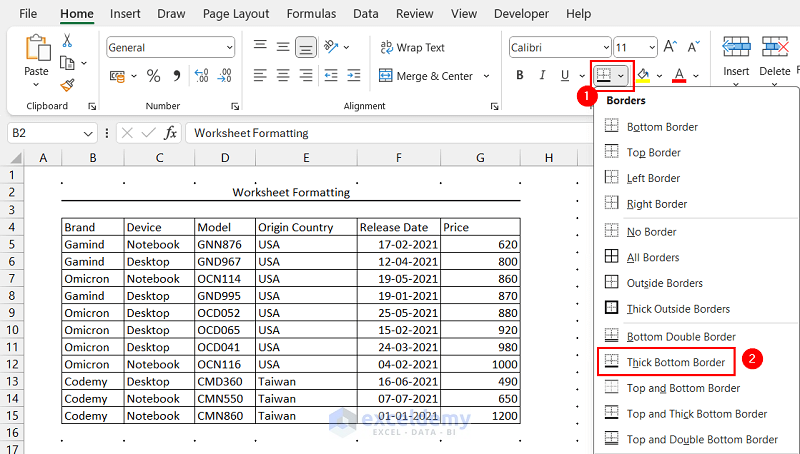
3.1 Apply Thick Bottom Border to Title

The Thick Bottom Border option is useful to differentiate between sections. Thus, applying this border to the title will visually separate the title from the data table.

To apply the Thick Bottom Border option in the title, follow the steps below:

1. Select the row where the title is displayed.
2. Click the Borders dropdown from the Font group.
3. Select the Thick Bottom Border option.

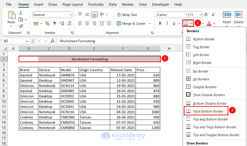
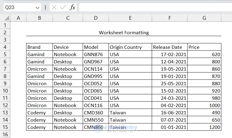
Now see, there is a thick bottom border in the title row.

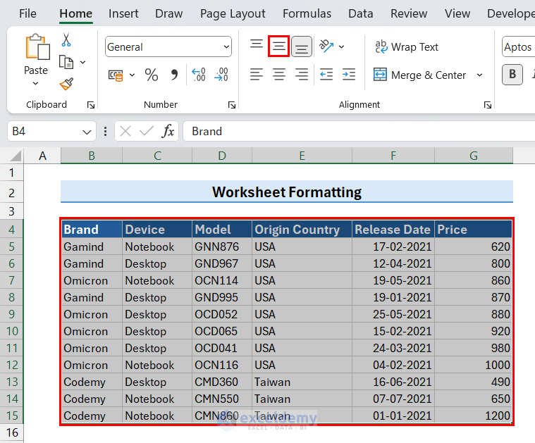
3.2 Apply All Borders Command

Here are the steps to apply the All Border command for the cells of the data table:

1. Select the data table.
   Here, I have selected the range B4:G15.
2. Click the Borders dropdown from the Font group.
3. Select the All Borders option.

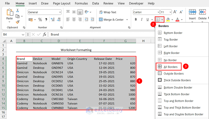
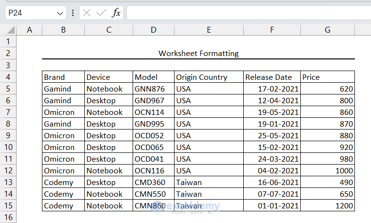
As you can see now, borders have appeared around each cell of the data table.

3.3 Change Border Color

The border color in Excel is set to black (automatic) by default. However, you may need a different border color based on the background color of the worksheet.

Here are the steps to change the border colors in an Excel worksheet:

1. Select the row with the title where the thick bottom border was applied.
2. Click Borders dropdown > Line Color > your preferred color.As a result, dot symbols will appear at each corner of cells throughout the worksheet.
3. Click the Borders dropdown again and select the Thick Bottom Border option.
4. This will change the border color of the row with the title.
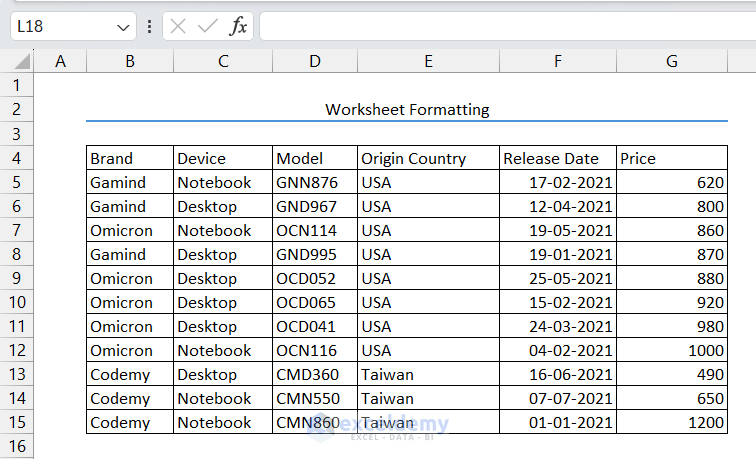
5. Similarly, change the border color of the data table as well.

4. Applying Cell Shading in an Excel Worksheet

You can apply fill color or cell shading to highlight important parts of the worksheet. In this section, we will apply cell shading to the title and column header rows to focus attention on these rows.

Here are the steps to apply cell shading in Excel:

1. Select the row with the title.
2. Click the Fill Color dropdown from the Font group.
3. Select a suitable color.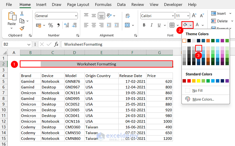As a result, the selected cell shading will appear in the title row.
4. Now, select the range with column headers.
   Here, I have selected the range B4:G4.
5. Click the Fill Color dropdown again and select your preferred color.

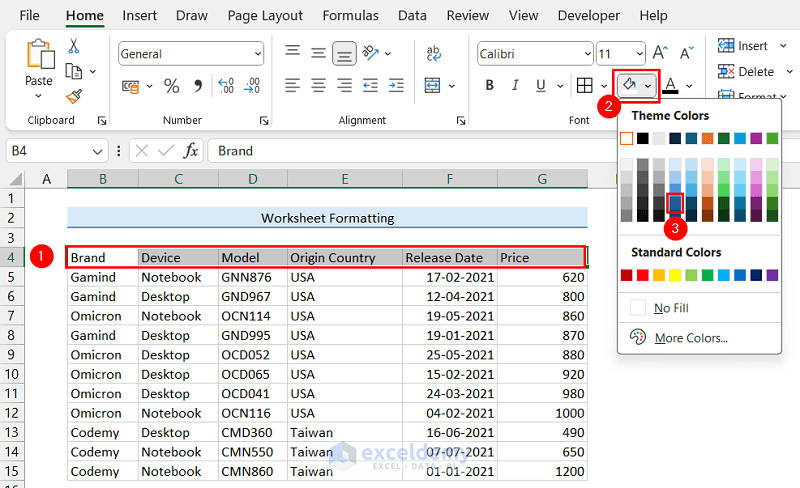
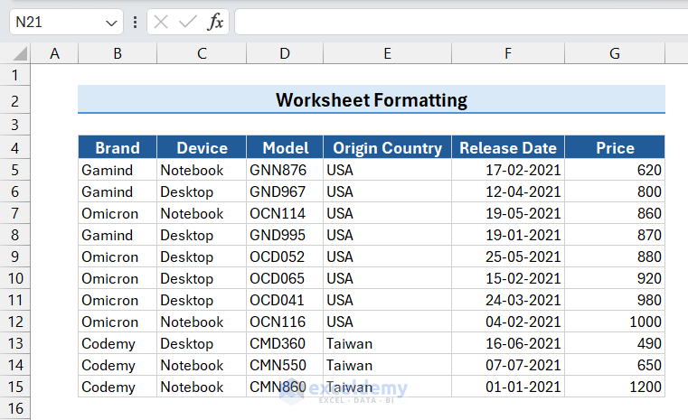
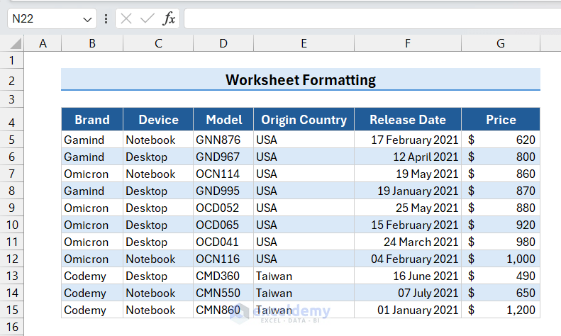
As a result, the title and column header rows will have a fill color like the following image. Using similar steps, you can apply cell shading to any range in a worksheet.

5. Changing Font Color in Excel

To properly format a worksheet, we should maintain color contrast between background color and font color. This helps to enhance the readability of data. In the previous section, we have picked a darker color in the column headers. Therefore, we should change the default back font color to a lighter color shade.

You can apply the steps below to change the font color of the column headers row:

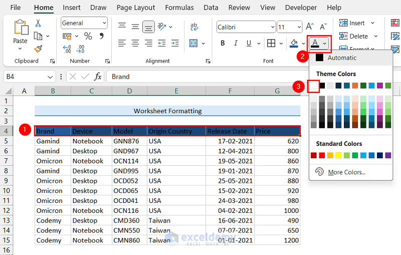
1. Select the row with column headers.
2. Click the Font Color dropdown from the Font group.
3. Select your preferred color.
   Here, I have selected the White color.
   

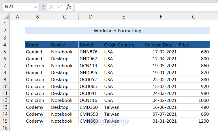
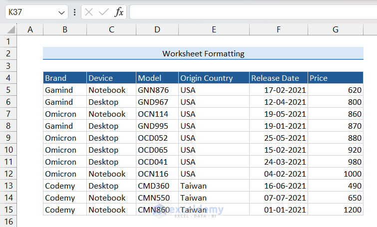
Now see, the font color of the column headers row has changed to White.

6. Changing Font in Excel

Proper use of font styles and font size helps to make any section of a worksheet stand out. By default, you will get Calibri font with 11 font size in Excel. However, this can be easily changed.

The following 2 examples will demonstrate how to change font size and font styles in Excel:

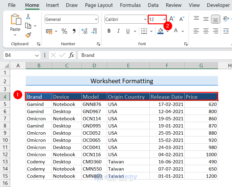
6.1 Change Font Size

In this example, we will change the font size of the title and column header rows to 14 and 12 respectively. Here are the steps to accomplish this:

1. Select the range with the title.
2. Click the Font Size dropdown and select 14.
   
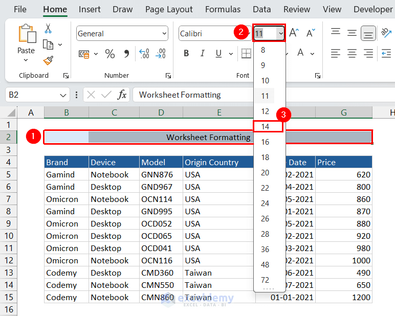
3. Similarly, select the column headers range and set the font size to 12.

6.2 Change Font Style

We will set the font style to bold for title and column header rows in this example. We will also change the font of the entire worksheet. Here are the steps to accomplish these:

1. Press and hold the Ctrl key while selecting the title range and column headers range (i.e. range B2:G2 and B4:G4).
2. Click the Bold command button.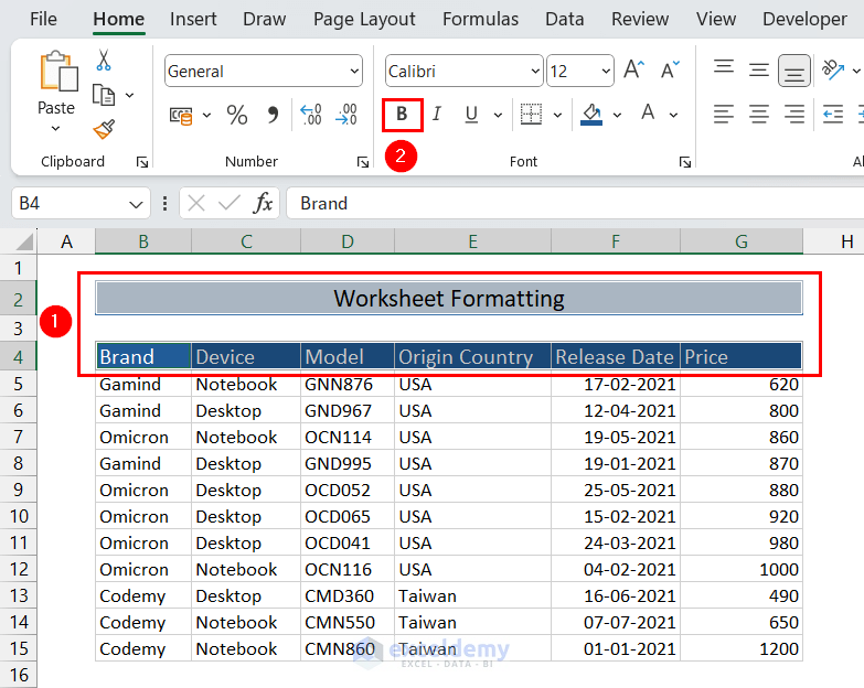This will change the font style of the selected ranges to bold.
3. Click the Select All button from the top-left corner of the worksheet.
4. Click the Font dropdown and select your preferred font.
   Here, I have selected the Aptos Narrow font.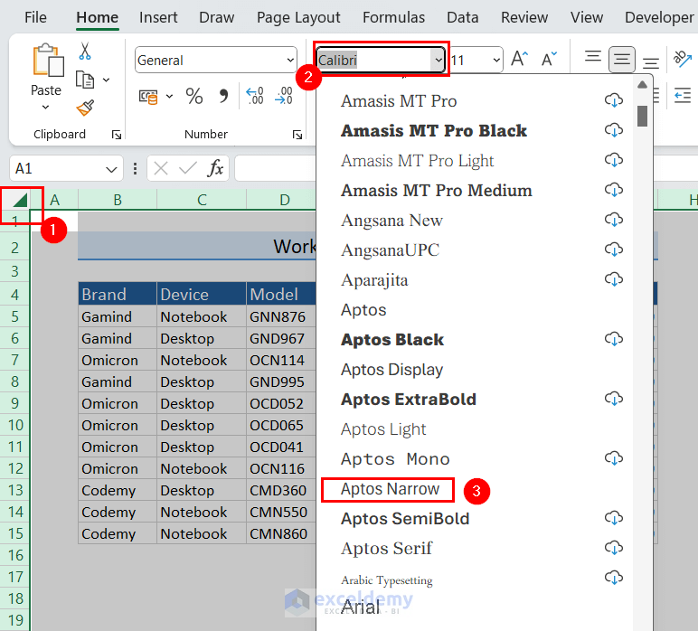

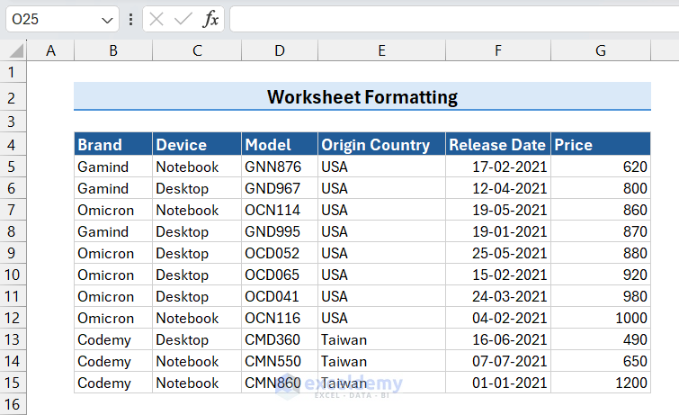
As you can see, the font in the worksheet has changed now.

Read More: Title in Excel

7. Changing Data Alignment in Excel

In Excel, there are two types of data alignment: horizontal and vertical. The horizontal alignment depends on the type of data. For example, texts are right-aligned whereas numbers and dates are left-aligned by default. The vertical alignment is set as Bottom Align usually.

However, you can easily change horizontal and vertical alignment options according to your worksheet formatting requirements. In this section, we will change the vertical alignment of the data table and the horizontal alignment of the column headers.

Here are the steps to change data alignment in a worksheet:

1. Select the data table (i.e. range B4:G15).
2. Click the Middle Align command from the vertical alignment options.
3. Afterward, select the column headers (i.e. range B4:G4).
4. Click the Center command from the horizontal alignment options.

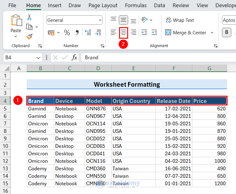
The data alignment in your worksheet has changed now.

8. Changing Number Format in Excel

Excel deals with different data types such as numbers, dates, times, percentages, currency, etc., and has multiple built-in number formats for these data types. You can also create a custom format to display the data in your preferred format.

Our sample worksheet contains dates formatted as dd-mm-yyyy in the Release Date column and numbers in the Price column. In the following two examples, we will change the number format of these two columns.

8.1 Modify Date Format

Here are the steps to change the date format in Excel:

1. Select the column with dates.
   Here, I have selected the range F5:F15.
2. Click the Format Cells dialog box launcher.
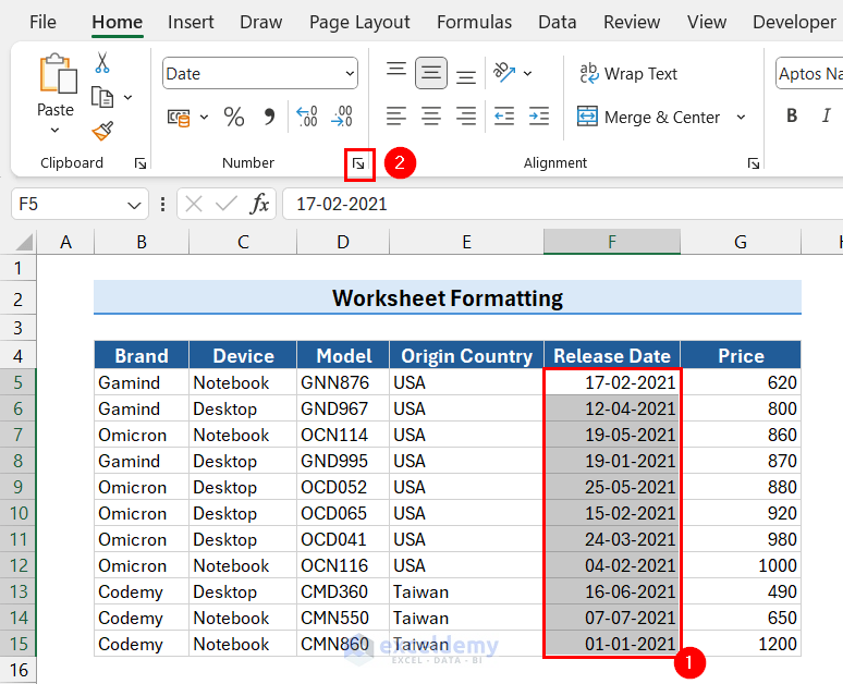   As a result, the Format Cells dialog box will appear.
3. In the Format Cells dialog box:
   • Go to the Number tab.
   • Select Date from Category.
   • Choose your desired data format.
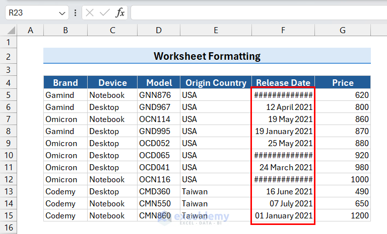
     Here, I have selected the dd mmmm yyyy format.
   • Click OK.

   

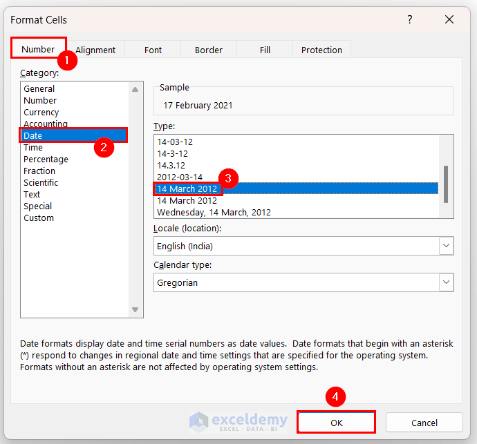
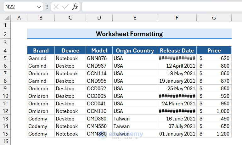
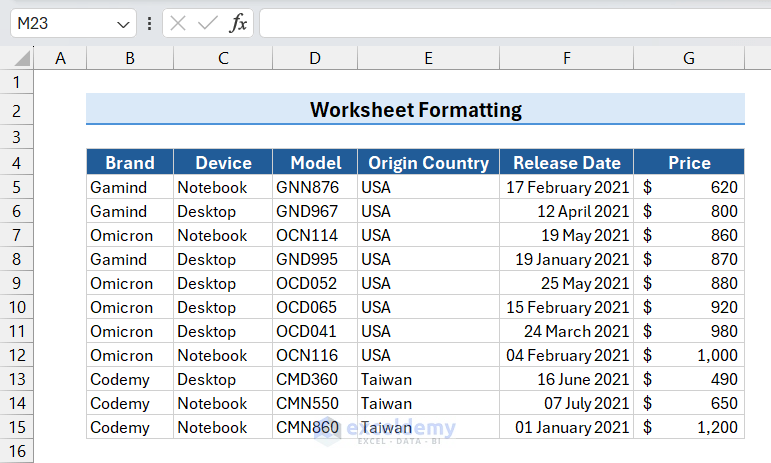
Now look, the selected date format has appeared in the target column. Although, you may notice ### symbols in some cells due to inadequate column width. We will discuss the process to fix this issue in the upcoming sections.

8.2 Apply Accounting Format

The price values can be displayed in Accounting or Currency format. In this example, we will apply the Accounting format. Here are the steps to accomplish this:

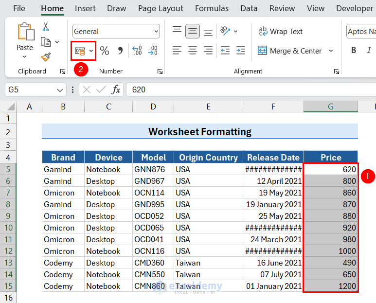
1. Select the column with price values.
   Here, I have selected the range G5:G15.
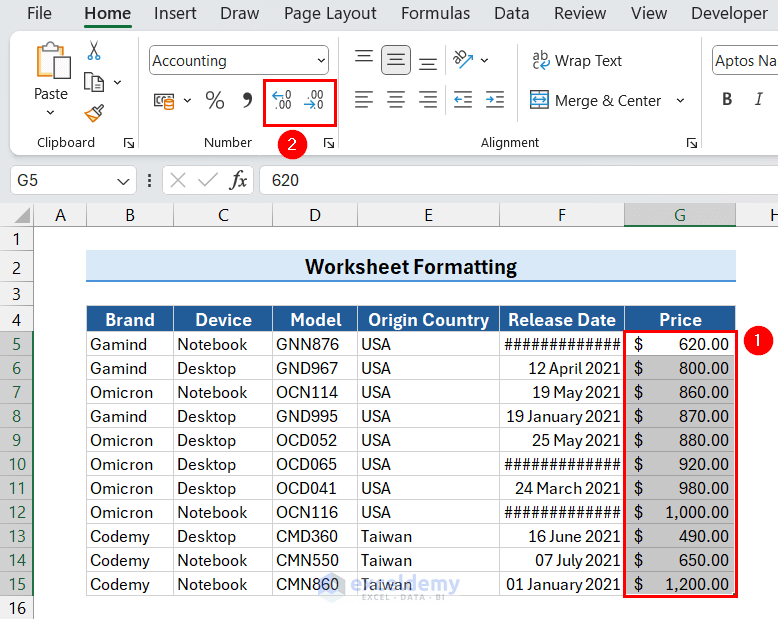
2. Click the Accounting format button.This will display the data in Accounting format.
3. If you want to change the number of decimal places, you click the Increase Decimal or Decrease Decimal buttons.

9. Changing Column Width in Excel

Sometimes you may ### symbols instead of actual values in some cells. It usually happens due to insufficient column widths. To fix this problem, you have to adjust the column width in Excel.

You can use the following 3 methods to adjust column width in Excel:

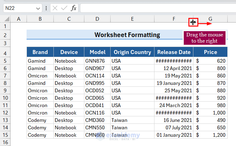
9.1 Use Mouse to Change Column Width

You can drag the column border with the mouse to adjust the column width. Here are the steps for that:

1. Hover the mouse pointer at the column bar’s right side in the desired column.
   As a result, the drag icon will appear.
2. Drag the column bar to the right until you get the desired width.

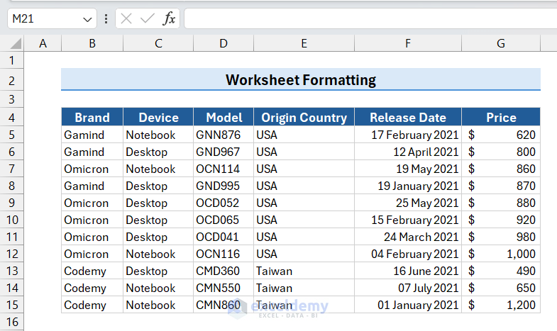
Now look, the column width is adjusted and the dates are appearing properly.

9.2 AutoFit Column

It is also possible to automatically adjust the column width. Here are the steps for that:

1. Hover the mouse pointer at the column bar’s right side in the desired column.
2. Double-click on the column bar’s right side.

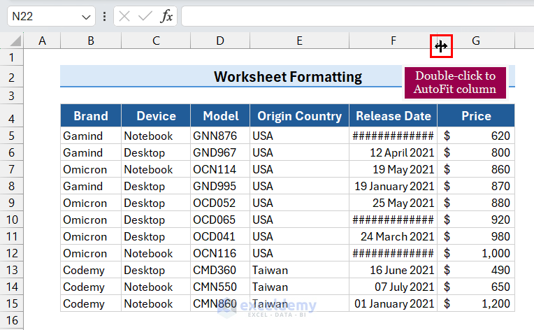
As a result, the column width will adjust automatically to fit the data in the column.

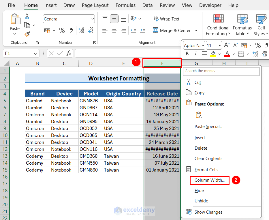
9.3 Set Column Width to a Specific Number

You can also set the column width to a specific number. Here’s how:

1. Select the desired column by clicking on the column bar.
2. Right-click on your mouse to open the context menu.
3. Select the Column Width option.
4. Enter the desired column width value in the Column Width dialog box and click OK.

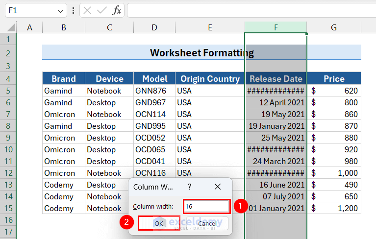
This will adjust the column width in your selected column.

10. Changing Row Height in Excel

When you add multi-line texts with the Wrap Text feature, the entire data may not be displayed due to insufficient row height. To fix that you can adjust row heights in your worksheet. You may adjust the row height to simply adjust the vertical spacing in a row as well.

The process of changing row height is similar to the changing column width process shown in the previous section. You can view the process in the following GIF:

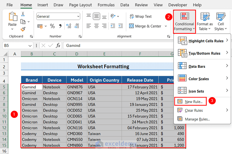
11. Applying Conditional Formatting in Excel

Conditional Formatting in Exel is used for formatting cells that meet a specific criterion. With this tool, various formatting can be added to a worksheet. In this example, we will apply alternative row colors in our worksheet using this tool.

Here are the steps to set alternative row colors by applying Conditional Formatting in Excel:

1. Select the rows for which you want to set alternative row colors.
   Here, I have selected the range B5:G15.
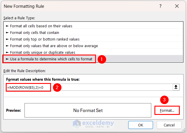
2. Click the Conditional Formatting dropdown and select the New Rule option.As a result, the New Formatting Rule dialog box will appear.
3. In the New Formatting Rule dialog box:
   • Select the rule type Use a formula to determine which cells to format.
   • Set the formatting rule to: =MOD(ROW(B5),2)=0
   • Click the Format button.

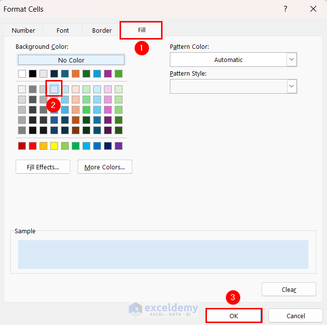
   This will open the Format Cells dialog box.

4. In the Format Cells dialog box:
   • Go to the Fill tab.
   • Select your preferred background color.
   • Click OK.

   

5. Now, you can preview the selected format in the Edit Formatting Rule dialog box. Finally, click OK in this dialog box as well.

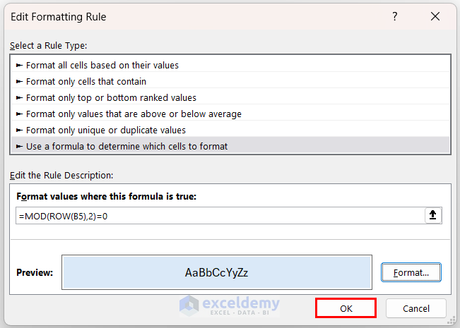
Now look, the alternative row colors are applied to the selected range in the worksheet.

Download Practice Workbook

Conclusion

To conclude our tutorial, we have covered 11 examples of formatting a worksheet. We used various Excel features to change gridlines, borders, fill color, font color, font alignment, number format, row height, and column width of our sample worksheet. You can use these examples to format your worksheet.
Thanks for reading this article. If you have any feedback or queries, let us know in the comment section.

Frequently Asked Questions

How do I quickly change the format of a worksheet?

Here are the steps to change the format of a worksheet quickly:

1. Go to the Page Layout tab.
2. Click the Themes dropdown.
3. Hover the mouse pointer over various themes to see the change in the worksheet format.
4. Select your preferred theme.

Can I copy formatting from one worksheet to another?

Yes, you can copy any worksheet format to other worksheets. Here are the steps to copy worksheet formatting to other sheets:

1. Select the cell or range whose formatting you want to copy.
2. Press the Ctrl+C keys to copy the cell.
3. Go to the target worksheet.
4. Select the cell or range where you want to paste the formatting.
5. Right-click on the mouse to open the context menu.
6. Select Formatting from the Paste Options.

How to freeze a row in a worksheet?

While working with worksheets containing a large dataset, we often need to freeze rows to keep specific rows visible when we scroll down. Consider a situation where you need to freeze the 5th row in a worksheet. Here are the steps to freeze that row:

1. Click the row bar of the 6th row.
2. Go to the View tab.
3. From the Freeze Panes dropdown, click the Freeze Panes option.

<< Go Back to Learn Excel