The Solver Add-in can solve linear and non-linear programming problems with multiple variables and constraints, whereas the graphical method can only be used to solve problems with two variables.
Click the image to get a detailed view
Download Practice Workbook
How to perform Linear Programming using the Solver in Excel
How to Add Excel Solver Add-in
The Excel Solver Add-in is not present in the Data tab by default.
- To add the Solver add-in from Excel Add-Ins, go to Data tab >> check if the Solver add-in is present >> go to the File tab if the Solver tool is not present.
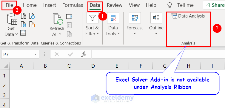
- Click Options.

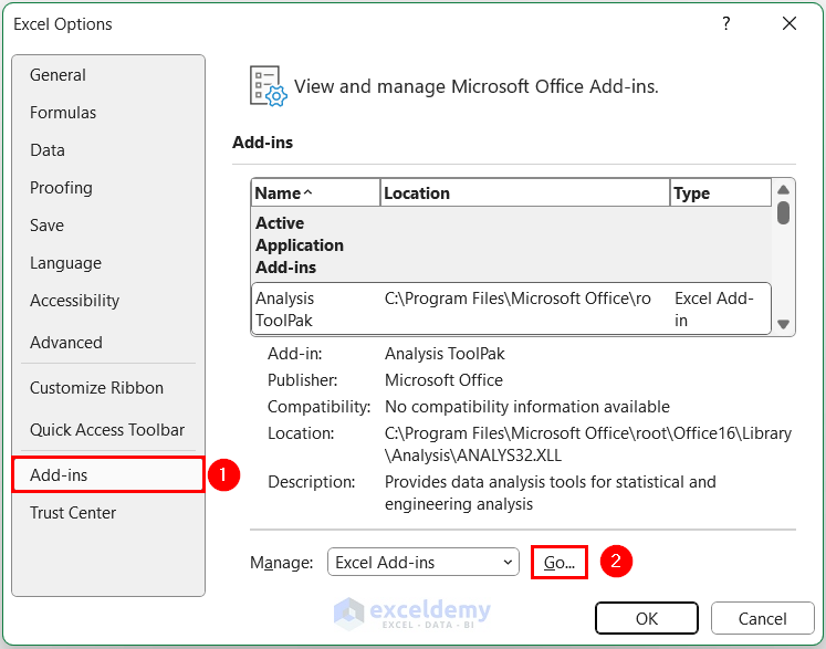
- In Excel Options, click Add-ins >> click Go.
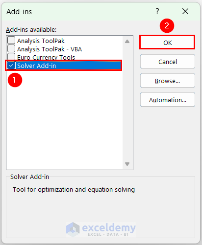
- In Add-ins, check Solver Add-in >> click OK . The Solver Add-in will be added to the Data tab.
How to Define and Formulate the Linear Programming Problem?
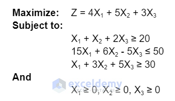
A linear programming problem consists of an objective function and some constraints. The objective function can be maximized or minimized.
To solve the following linear programming model which has an objective function Z, which you want to maximize, and 3 different constraints for the X1, X2, and X3 variables.
How to Tabulate Linear Programming Problems in Excel
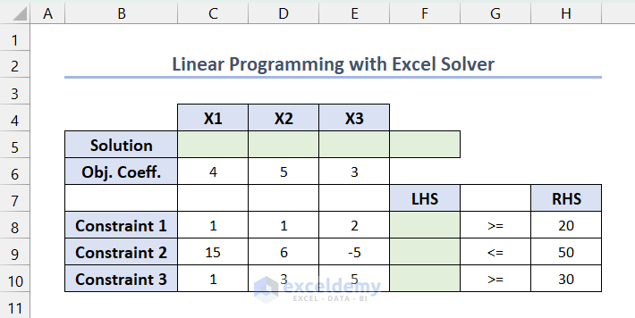
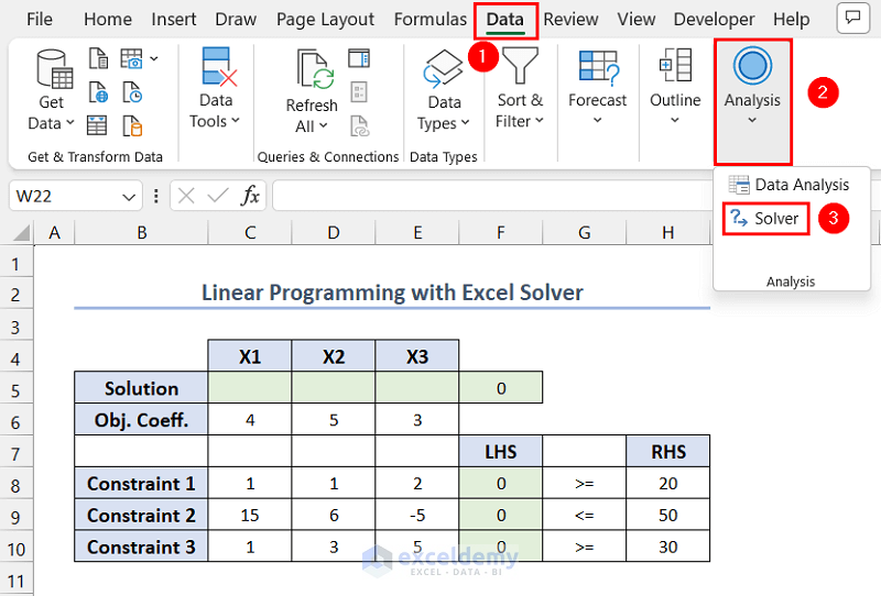
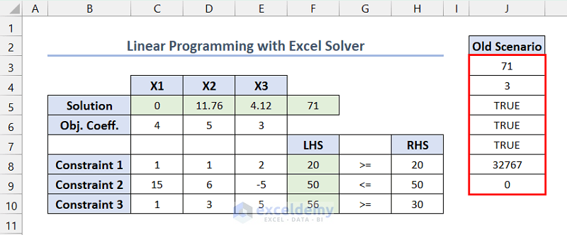
- Tabulate the linear programming model in the following format to input the objective functions and constraints in the Excel Solver Add-in. Here, the Light Green colored boxes are kept empty for calculations and solutions.
- Use the following formula in F5. The range C5:E5 is empty, so F5 shows 0. This value indicates the current value of the objective function.
=SUMPRODUCT(C5:E5,C6:E6)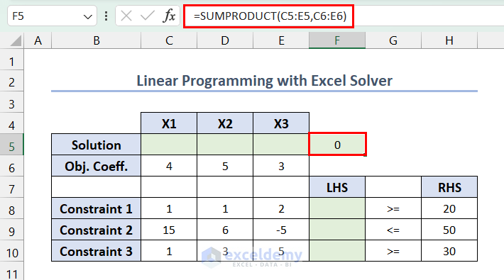
- For the constraints, enter the following formula in F8 >> press Enter >> drag down the Fill Handle.
=SUMPRODUCT($C$5:$E$5,C8:E8)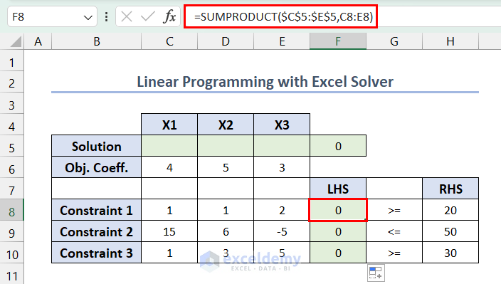
How to Solve a Problem Using the Excel Solver
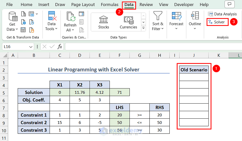
- Go to the Data tab >> click Analysis >> select Solver.
Click the image for a detailed view
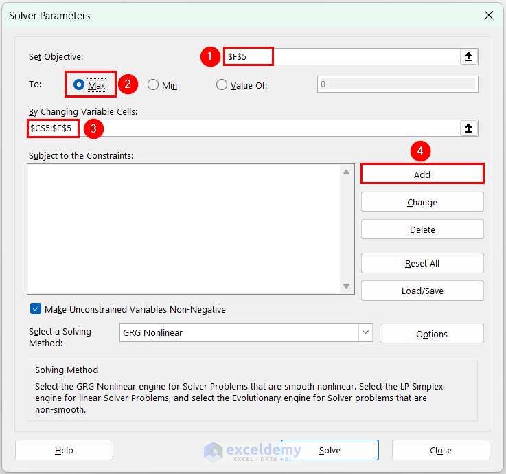
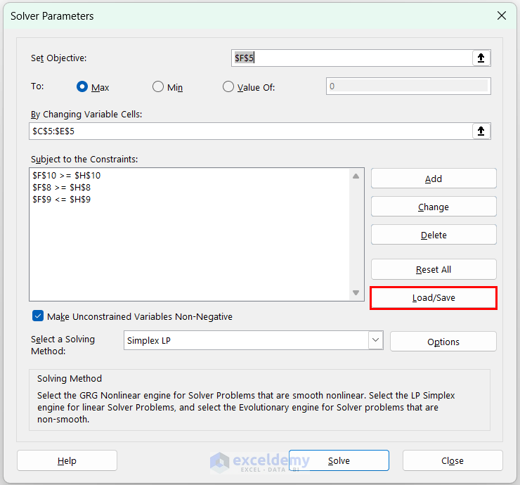
- In Solver Parameters, enter $F$5 in Set Objective >> In To, click Max >> In By Changing Variable cells, select the range $C$5:$E$5>> click Add to add constraints.
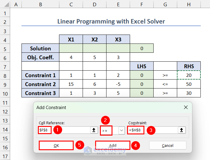
- In Add Constraint, enter $F$8 in Cell Reference >> select >= operator for the first constraint >> Enter $H$8 in Constraint >> click Add to add constraints 2 and 3 >> click OK.
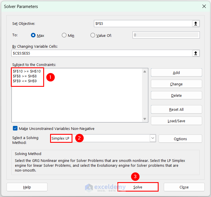
- Constraints were added to Subject to the Constraints. In Select a Solving Method >> select Simplex LP >> click Solve.
The required values for the variables and the objective function for the linear programming maximization problem will be displayed.
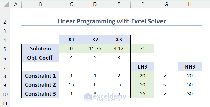
Here, the maximized value of the objective function is 71, and the values for the variables X1, X2, and X3 are 0, 11.76, and 4.12.
Read More: How to Find Optimal Solution with Linear Programming in Excel
How to Save and Load Solver Scenarios in Excel
- To save a linear programming model, select a range to input the variable values >> go to the Data tab >> click Solver.
Click the image for a detailed view
- In Solver Parameters, you can see the last solved model. Click Load/Save.
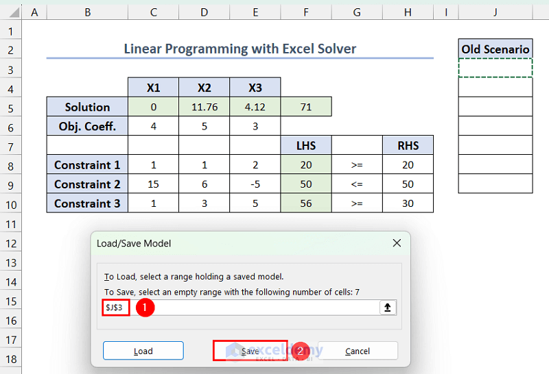
- In Load/Save Model, provide the reference of the first cell in the selected range ($J$3, here) >> click Save.
Click the image for a detailed view
You will see the linear programming model variable values in the selected range.
Click the image for a detailed view
How to Load the Saved Model
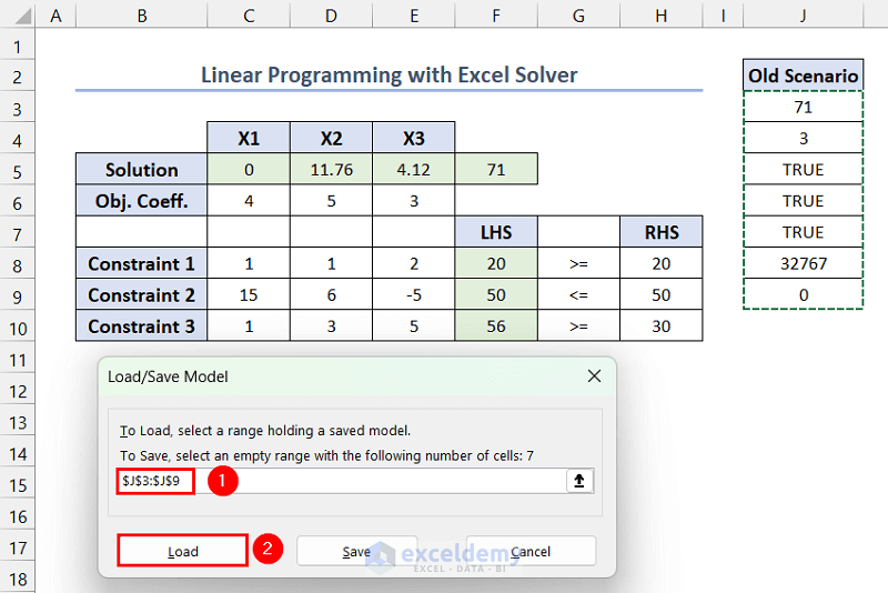
- In Solver Parameters, click Load/Save >> select the range containing the previous model ($J$3:$J$9, here) >> click Load.
Click the image for a detailed view
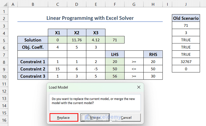
- In Load Model, click Replace.
Click the image for a detailed view
The Solver Parameters user form will open and replace the existing model parameters with the loaded model parameters. Click Solve to recalculate it.
How to perform Linear Programming Using the Graphical Method in Excel
How to Define and Formulate the Problem
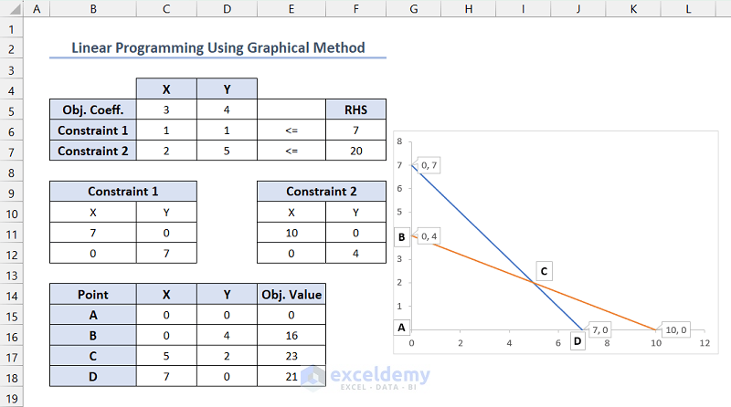
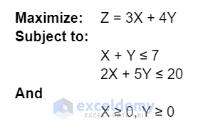
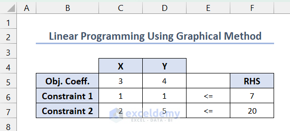
- Define an objective function and constraints for the linear programming problem. Here, the linear programming model has an objective function Z, which you want to maximize, and 2 different constraints for the X and Y variables.
How to Tabulate the Linear Programming Problem in Excel
- Tabulate the linear programming model in the following format using the variable coefficients.
Read More: How to Do Linear Programming in Excel
How to Plot a Chart Using the Constraints
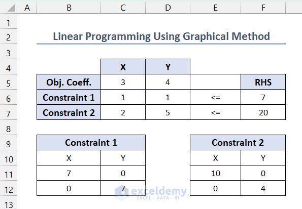
- Calculate the X and Y-axis intersection points for each constraint by setting one variable equal to zero. For example, for the first constraint, if Y = 0 then X = 7, and if X = 0 then Y = 7.
- List these intersection points for each constraint in the following format.
- Select the intersection points of constraint 1 >> go to the Insert tab >> Select Scatter >> choose Scatter with Smooth Lines.
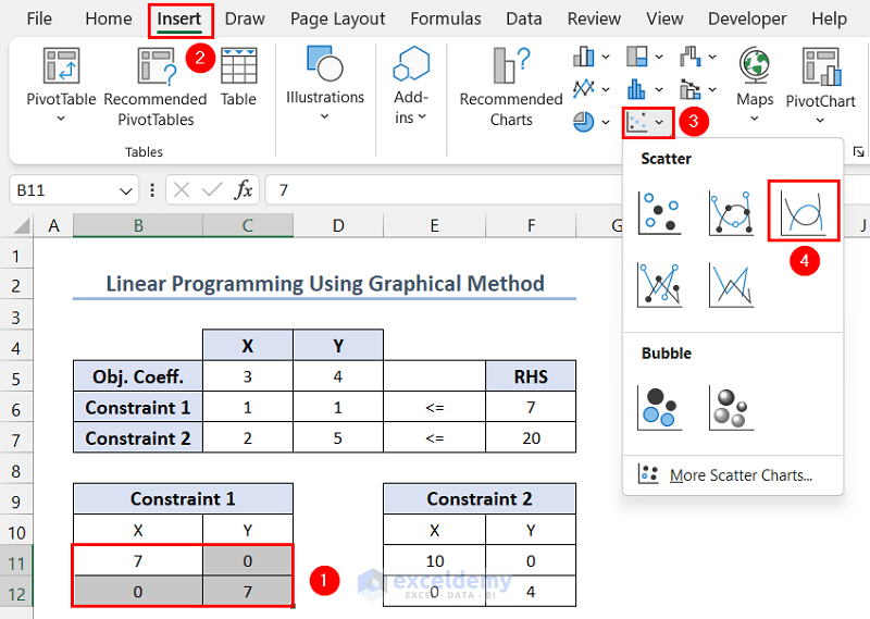
Click the image for a detailed view
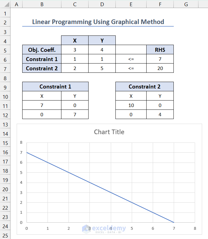
A chart like the following will be displayed.
- Select the chart and right-click >> click Select Data.
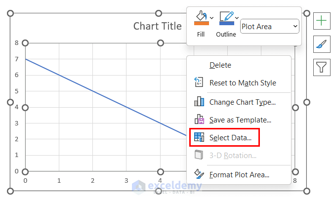
- In Select Data Source, select Series 1 and click Edit.
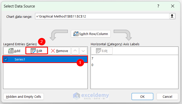
- In Edit Series, set the Series Name to range $B$9:$C$9 and click OK .
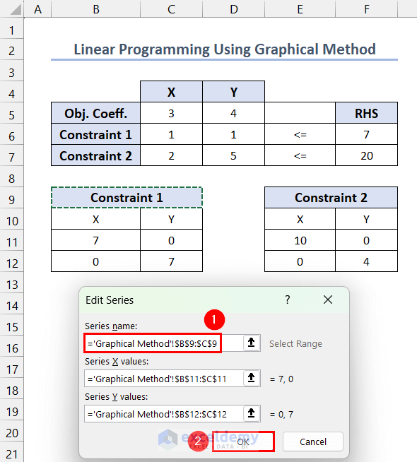
- Click Add.
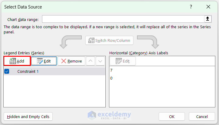
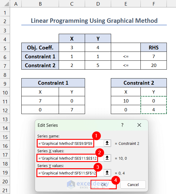
- Set the Series Name to $E$9:$F$9 >> Series X Values to $E$11:$E$12 >> Series Y Values to $F$11:$F$12 >> click OK.
- In Select Data Source, click OK.
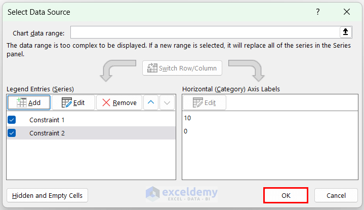
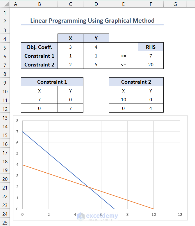
The chart for the constraint lines is displayed.
- Select the chart and click the plus (+) icon to view the Chart Elements >> check Data Labels >> click the right side of Data Labels to see additional options >> click Data Callout option to see X and Y-axis intersection points >> uncheck Gridlines to remove grids.
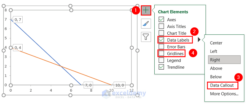
Click the image for a detailed view
How to Determine the Coordinates of Each Corner Point in the Feasible Region
Since both the constraints have a <= (less than or equal to) operator and X, Y values are greater than or equal to zero, the marked ABCD region is your feasible region. (Here, A B C D were manually placed to show the corner points)
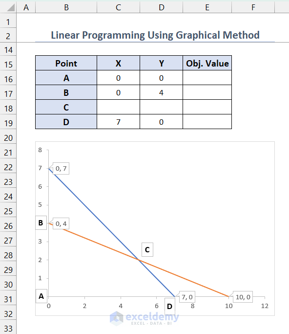
- List all the corner points (A, B, C, and D) of the feasible region and calculate the objective function value in those points. You can get the X and Y values for A, B, and D from Data Callouts.
- To calculate X and Y values for point C, use the following formula in C17.
=TRANSPOSE(MMULT(MINVERSE(C6:D7),F6:F7))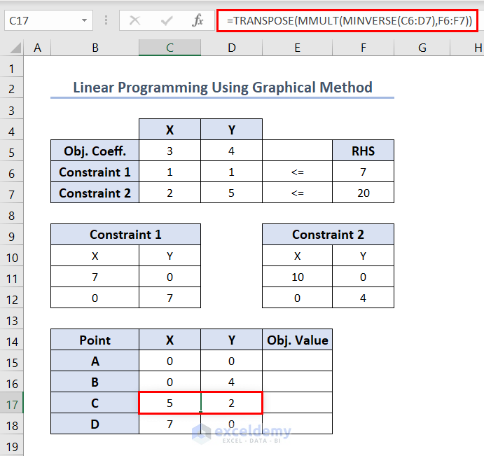
Here, the MINVERSE function calculates the inverse matrix of the matrix formed with X and Y value coefficients in constraints (range C6:D7). And the MMULT function multiplies that inverse matrix with another matrix (range F6:F7). Finally, the TRANSPOSE function converts the rows into columns and columns into rows for the output returned by the MMULT function.
Read More: How to Find Optimal Solution with Linear Programming in Excel
How to Calculate the Value of the Objective Function for Each Corner Point?
- Enter the following formula in E15 >> press Enter >> use the Fill Handle tool.
=SUMPRODUCT($C$5:$D$5,C15:D15)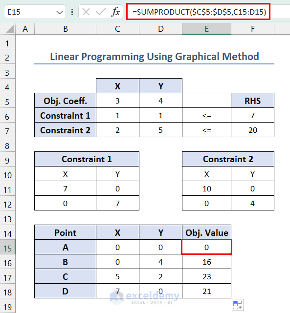
The maximum value occurred in point C. And the value of the maximized objective function is 23.
Read More: How to Solve Blending Linear Programming Problem with Excel Solver
Frequently Asked Questions
1. What are the limitations of using the Excel Solver for Linear Programming?
Answer: Although Excel Solver Add-in is a powerful tool, it has limitations:
>> it is suited for small to medium-sized linear programming problems (up to 200 variables)
>> it operates with limited precision (up to 15 decimal points)
>> it operates with very few numbers of algorithms (Simplex Method for Linear Programming Problems), etc.
2. Can I use the graphical method to solve Linear Programming Problems with 3 variables?
Answer: If we apply the graphical method for Linear Programming problems with 3 variables, the feasible region will be a 3-dimensional space. Since representing 3-dimensional space on a two-dimensional plane can be complex and visually overwhelming, the graphical method is not suitable for Linear Programming problems with more than two variables.
3. Are there any alternative tools or software besides Excel Solver to solve Linear Programming problems?
Answer: There are some alternative tools or software:
>> IBM ILOG CPLEX optimizer
>> MATLAB Optimization Toolbox
>> GNU Linear Programming Kit
>> PuLP, etc.
Excel Linear Programming: Knowledge Hub
- How to Solve Integer Linear Programming in Excel
- How to Calculate Shadow Price Linear Programming in Excel
- How to Perform Mixed Integer Linear Programming in Excel
- How to Do Linear Programming with Sensitivity Analysis in Excel
- How to Graph Linear Programming in Excel
<< Go Back to Solver in Excel | Learn Excel
Get FREE Advanced Excel Exercises with Solutions!

Excel Linear Programming (Using Solver and Graphical Methods)
I thought this article was made extremely well. It showed how to install the necessary tools, how to use linear programming on excel (step by step) and also showed other excel solver alternatives such as IBM ILOG CPLEX optimizer. The only thing that I would like added to this article is an example along with the step-by-step tutorial just to add context to the steps. I would like to apply these models in figuring out problems such as how many units of product A and B should we produce to maximize profit?
Hello Martin,
We are glad to hear that you found this article useful! Including a real-life example in tutorials can indeed make the steps more relatable and easier to understand. Applying these models to specific scenarios like maximizing profit by determining the production units for products A and B is a great way to leverage linear programming. We will include this in our next update.
Regards
ExcelDemy