How to Utilize Solver for Optimization in Excel (6 Methods)

Understanding Solver in Excel

Solver acts as a specialized tool that you can incorporate into programs like Excel, functioning as an add-in. Its primary purpose is to solve intricate problems by employing mathematical methods to find the best solution. Solver is particularly adept at resolving linear programming problems, which involve maximizing or minimizing a value while adhering to certain constraints.

This capability has led some individuals to refer to it as a linear programming solver. However, its utility extends beyond linear problems; it can also address other types of challenges involving curves and complex scenarios.

Thus, whether your problem is straightforward or intricate, Excel Solver is equipped to lend assistance.

Enabling Solver in Excel

To activate Solver in Excel, follow these steps:

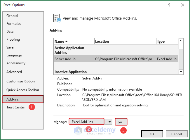
• Open the Excel Options window by clicking on File and selecting Options.
• Select Add-ins from the panel on the left.
• Choose Excel Add-ins in the Manage dropdown menu and click on Go…

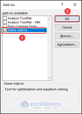
• In the Add-ins dialog box, check the box next to Solver Add-in and click OK.

Method 1 – Utilizing Solver for Optimization Without Constraints

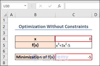
In this method, we aim to minimize the value of ()=3+32−5f(x)=x3+3x2−5 without any constraints.

• Enter the formula =43+3∗42−5=C43+3∗C42−5 in cell C7 to represent the equation of $f(x)$, where $C4$ denotes the value of $x$.

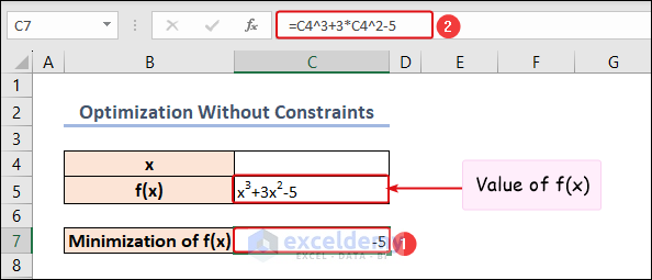
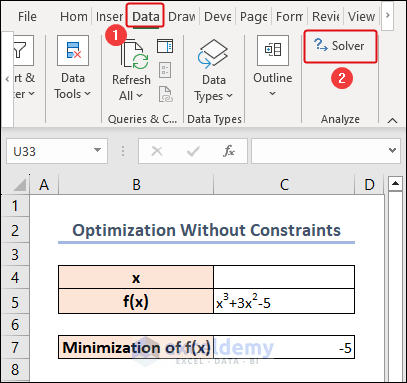
• Navigate to the Data tab and select Solver from the Analyze group.

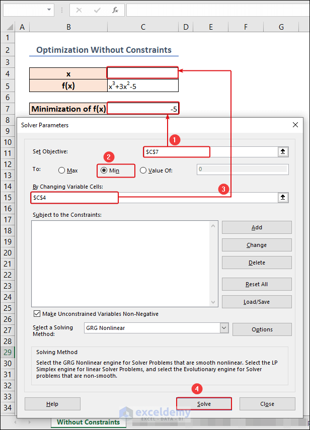
• In the Solver Parameters dialog box:
  • Set Objective: Select cell C7 and choose Min.
  • By Changing Variable Cells: Select cell C4.
  • Click Solve.

The value of x in cell C4 is converted to 0 and the minimum value of f(x) is achieved.

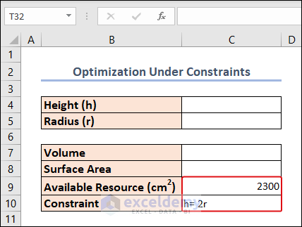
Method 2 – Optimization Under Constraints with Solver in Excel

Here, we introduce constraints to the optimization process using Solver.

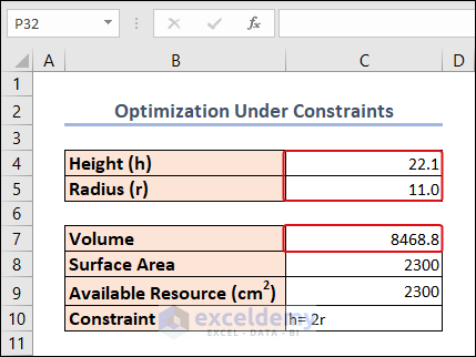
To explain this method, we have 2300 cm² of metal sheet in our hand. From this, we have to make a cylinder with a Height double its Radius. We have to optimize the system so that the Volume gets maximized.

• Calculate the Volume (V) using the formula =2ℎV=πr2h in cell C7, where $\pi$ denotes the constant value of pi (3.1416), $C4$ and $C5$ represent the height and radius, respectively.

• Determine the Total Surface Area (A) of a cylinder using the formula $A=2\pi r(h+r)$ in cell C8.

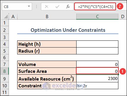
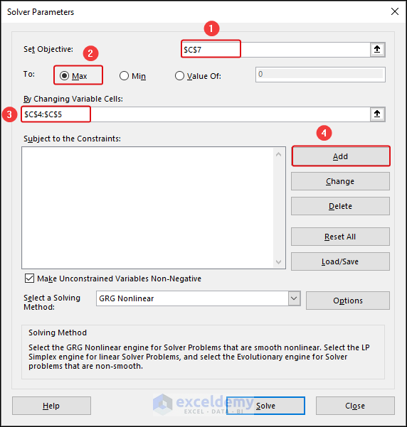
In the Solver Parameters dialog box:

• Set Objective: Choose Min for cell C7.
• By Changing Variable Cells: Select cells C4 and C5.
• Add Constraints: Ensure that the height is twice the radius, and the total area does not exceed the given metal sheet area.

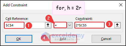
• • In the Add Constraint dialog box, select C4 as Cell Reference, select the Equal sign, and insert the following in the Constraint box.

• Click on Add for adding more constraints.

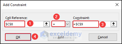
• Select C8 as Cell Reference, select the Equal sign, and select cell C9 in the Constraint box.
• Click OK.

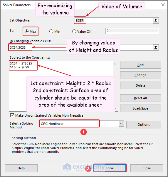
• You can find the added constraints in the Subject to the Constraints box in the following image.
• Select GRG Nonlinear in the Select a Solving Method section and click Solve.

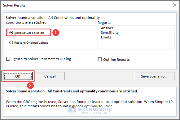
• In the Solver Results dialog box, check the Keep Solver Solution option and click OK.

The maximum achievable Volume with this area of the metal sheet is visible in cell C7 and its Height and Radius are also available.

Method 3 – Maximizing Profit by Optimization in Product Mix

In this scenario, we maximize profit by determining the quantity of each product to be produced while considering resource constraints.

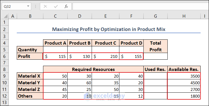
• The profit for each product of 4 types is displayed in the C6:F6 range.
• The required amount of material for each product type is available in the C9:F12 range.
• The available amount of each material is here under the Available Resource column (Column H).

Now, we’ll calculate the quantity of each product to be produced using the given resources. Our prime objective is to maximize the profit from this production.

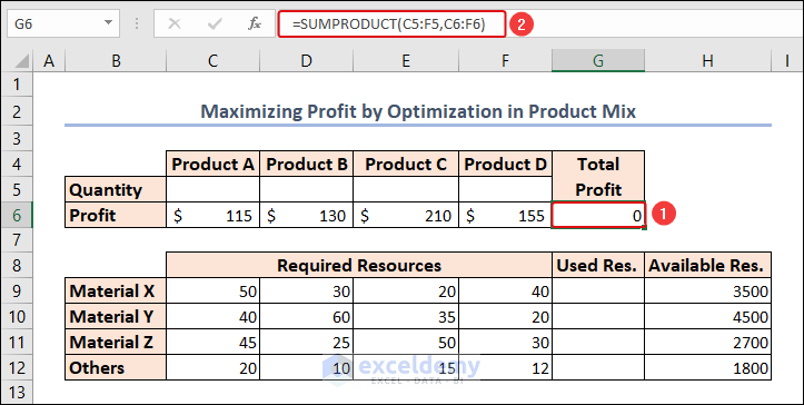
• To Calculate the Total Profit using the SUMPRODUCT function in cell G6.

The SUMPRODUCT function returns the sum of the products of the corresponding values from all the arrays.

• Compute the Total Resource Usage for each material in cell G9.

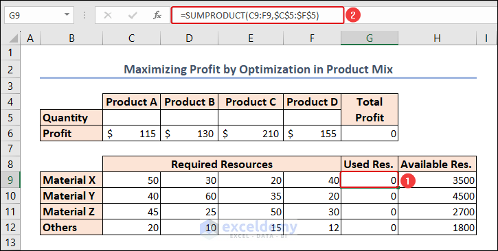
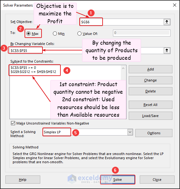
In the Solver Parameters dialog box:

• • Set Objective: Choose Max for the Total Profit (G6).
  • By Changing Variable Cells: Select the cells representing product quantities (C5:F5).
  • Add Constraints: Ensure non-negativity and resource availability.  The constraints are described in the image, and we selected the Simplex LP method for solving.
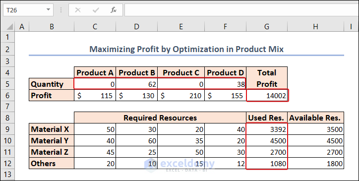
  • Click Solve.

At a glance, Excel computed the quantity of products, utilized resources, and the maximum total profit.

Read More: How to Calculate Optimal Product Mix in Excel

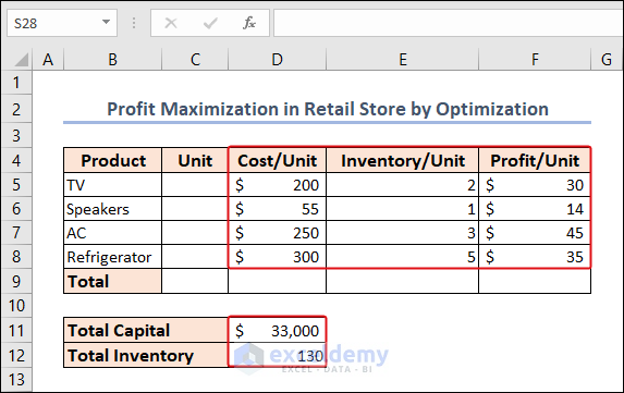
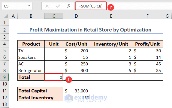
Method 4 – Profit Maximization in Retail Stores with Optimization

• We have several products from a retail electronics store.
• There are cost/unit, inventory/unit, and profit/unit are available under columns D, E, and F.
• The total capacity of inventory and the total capital (cash in hand) are given in the D11:D12 range.

Our aim is to maximize the profit while considering inventory and capital constraints in a retail setting.

Calculate the total unit of products, total cost, inventory, and profit:

• The total unit of products is calculated using the following formula in cell C9.

The SUM function adds all the numbers in each range of cells.

• The total cost is calculated with the following formula in cell D9.

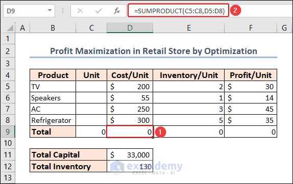
Similarly, the total inventory and total profit is calculated in cells E9 and F9.

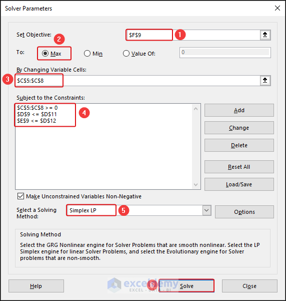
In the Solver Parameters dialog box:

• • Set Objective: Choose Max for total profit (F9).
  • By Changing Variable Cells: Select cells representing product quantities (C5:C8).
  • Add Constraints: Ensure non-negativity and resource availability. The total cost of buying products should be less than the total capital (cash in hand). The total occupied inventory should be less than the total available inventory.
  • We selected the Simplex LP method for solving.
  • Click Solve.

So, we can see that, the only way to make the most profit is by buying ACs. However, the inventory needs to be expanded as only one-third of the capital can be spent.

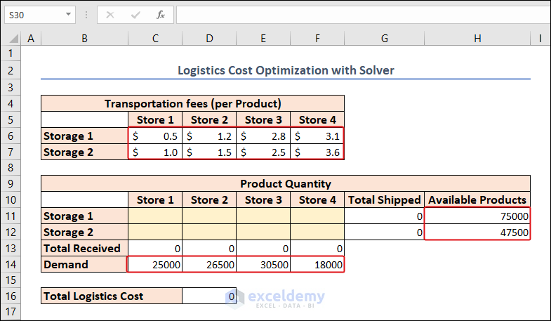
Method 5 – Logistics Cost Optimization with Excel Solver

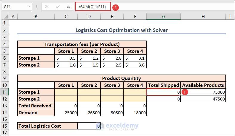
• In the C6:F7 range, we have the transportation fees for 4 different stores from 2 different storage houses.
• The available products in each storage are also available in the H11:H12 range.
• We can also find the demand for each store (retail store) in the C14:F14 range.

We should meet the demand of each store and make the logistics cost the bare minimum.

Calculate the total shipped products from each storage and received products for each store.

• The following formula in cell G11 determines the total shipped products from Storage 1.

• Use the same formula for Storage 2 in cell G12.

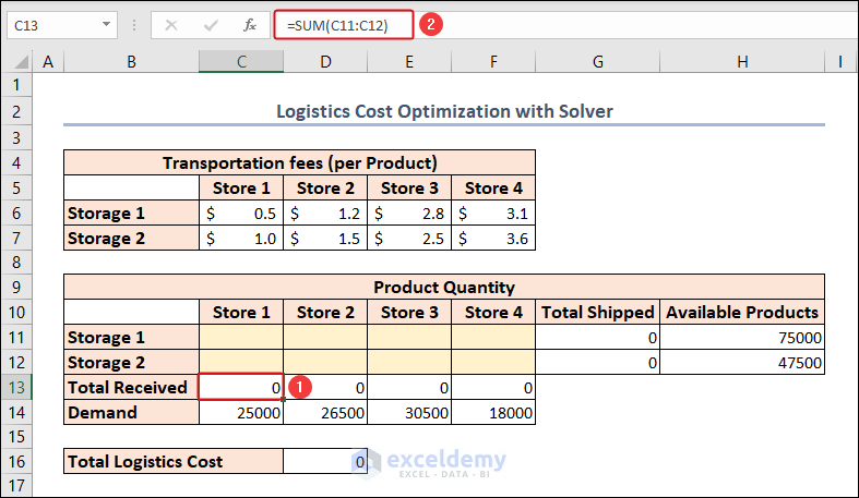
• For calculating the total received products of Store 1 from both storages, enter the following formula in cell C13:

• Use the same formula for the 3 remaining stores in cells D13:F13.

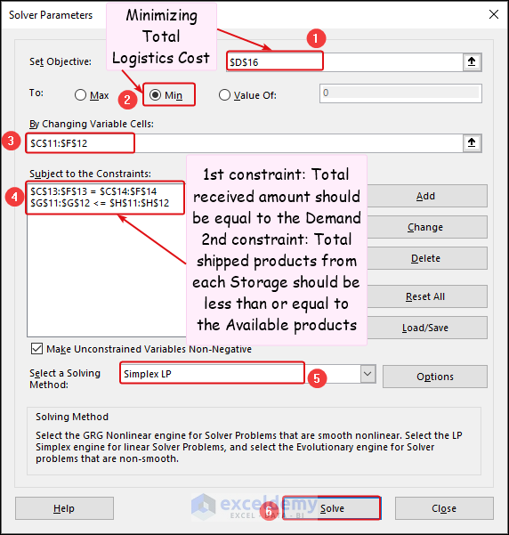
In the Solver Parameters dialog box,

• Select cell D16 in the Set Objective box and choose Min in the To section.
• In the By Changing Variable Cells box, select cells in the C11:F12 range.
• Constraints are described in the following image and we selected the Simplex LP method for solving.
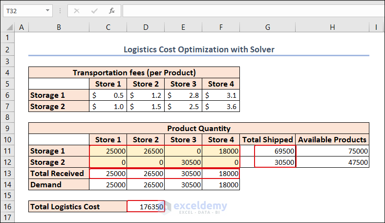
• Click Solve.

Our optimization in Excel is done.

Method 6 – Create Magic Square with Solver in Excel

What is Magic Square?

A magic square is like a puzzle that consists of a square grid. You can imagine it as a square box divided into smaller boxes or cells. Each cell in the grid contains a different number, usually a whole number.

The remarkable thing about a magic square is that if you add up the numbers in any row (going from left to right), any column (going from top to bottom), or either of the two main diagonals (the diagonal lines that go from one corner of the square to the opposite corner), the total will always be the same.

It’s like magic because the sum will always be equal no matter which row, column, or diagonal you choose.

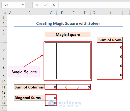
How to Create Magic Square

Here, we opt to create a 4*4 magic square:

• So, there would be 1 to 16 numbers in the 16 different cells.
• We calculated the sum of rows in the H6:H9 range.
• There is the sum of columns in the C11:F11 range.
• The diagonal sums are in the C13:C14 range.

For a 4*4 magic square, the sum for any columns or rows has to be,

Here, n represents the size of the magic square, which is the number of cells in each row or column.

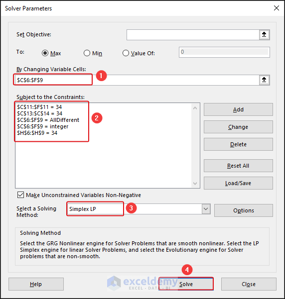
In the Solver Parameters dialog box, we inserted the following constraints as in the image below:

• Set Objective: Choose Min for a cell representing the deviation from the target sum.
• By Changing Variable Cells: Select cells representing the magic square values.
• Add Constraints: Ensure the sum of rows, columns, and diagonals equals the target sum.
• Click Solve.

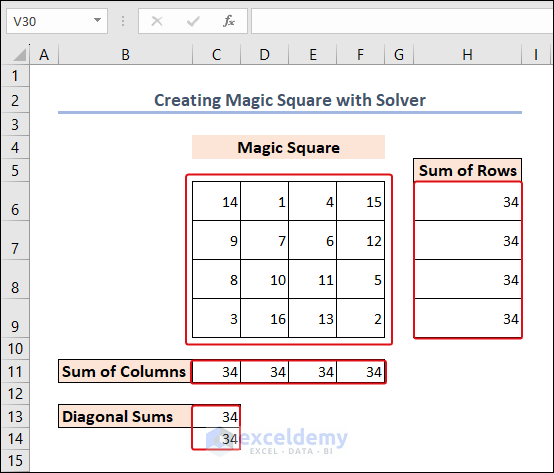
Magically, Excel created the magic square. You can apply the same procedure for magic squares of any dimension.

Excel Solver Algorithms

Different solving methods in Excel Solver cater to various problem types:

GRG Nonlinear: This method utilizes the Generalized Reduced Gradient (GRG) Nonlinear algorithm. It is specifically designed for tackling problems that involve smooth nonlinear functions. In other words, if your problem includes at least one constraint that is a smooth nonlinear function of the decision variables, this method can be useful.

LP Simplex: The LP Simplex method is based on the Simplex algorithm, which was developed by an American mathematician named George Dantzig. It is employed for solving Linear Programming (LP) problems. Linear Programming deals with mathematical models where the requirements can be described by linear relationships. These models usually consist of a single objective represented by a linear equation that needs to be either maximized or minimized.

Evolutionary: The Evolutionary method is suited for non-smooth problems, which are generally the most challenging type of optimization problems to solve. Non-smooth problems often involve functions that are not smooth or even discontinuous. In such cases, determining the direction in which a function is increasing or decreasing becomes difficult. The Evolutionary method is tailored to handle these complex optimization problems.

By selecting the appropriate solving method based on the nature of your problem, you can leverage the power of Excel Solver to find optimal solutions efficiently.

Things to Remember

• Enable the Solver Add-in before starting optimization.
• Select the appropriate solving method based on the problem type.
• Press Esc to halt Solver if needed.

Frequently Asked Questions

1. What is the objective function in optimization?

The objective function represents the quantity to maximize or minimize in optimization.

2. What are the constraints in optimization?

Constraints limit the feasible solutions in an optimization problem.

3. Can Excel Solver handle large-scale optimization problems?

While Excel Solver can handle moderately large problems, specialized software may be needed for very large-scale or complex problems.

Download Practice Workbook

You can download the practice workbook from here:

Optimization in Excel: Knowledge Hub

<< Go Back to Solver in Excel | Learn Excel