Linear optimization is one of the key topics of statistics. We can perform predictive analysis using the variables’ available data. In the following article, with easy steps, we will show to you how you can solve a linear optimization model in Excel.
What Is Linear Optimization?
In a mathematical model, linear optimization is a technique to get the optimal result, such as the highest profit or the lowest price. The requirements for linear optimization are represented by linear relationships. All types of linear optimization models include some main factors. They are given below:
- Decision Variables: We determine the decision variables that minimize or maximize the objective function.
- Objective Function: This is a function that helps us to determine the decision variables. It expresses the relation between the result and the variables.
- Constraints: Constraints are also functions that denote different conditions on possible solutions.
How to Solve Linear Optimization Model in Excel: 4 Easy Steps
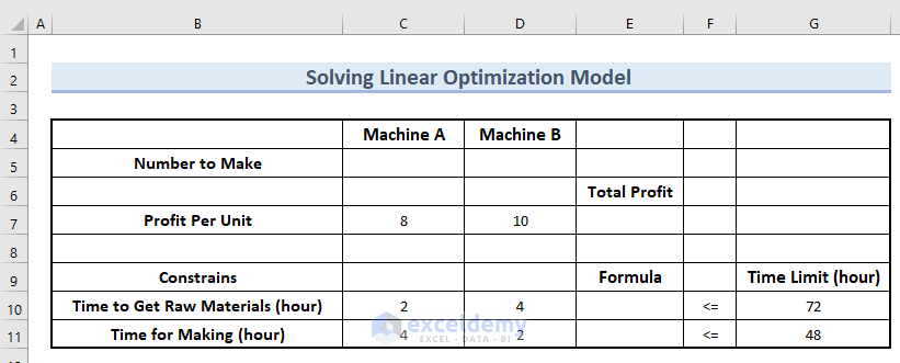
Suppose, we have two types of machine, Machine A and Machine B. The Profit Per Unit of Machine A is $8 and for Machine B is $10. Here, Time to Get Raw Materials for Machine A is 2 hours, and for Machine B is 4 hours. Along with that, Time for Making Machine A is 4 hours, and Machine B is 2 hours. If we have a total of 72 hours to Get Raw Materials and a total of 48 hours for making, then what are the maximum number of Machine A and Machine B that can be produced to make the maximum profit?
In the following article, we will describe 4 easy steps to solve the above linear optimization models in Excel. Here, we used Excel 365. You can use any available Excel version.
Step-1: Analyzing the Question
Here, according to the given problem, we have made the following dataset. Next, we will find the optimum Machine A number in cell C5, and the optimum Machine B number in cell D5.
Along with that, we will find the maximum Total Profit in cell E7.
Now, let us describe the problem thoroughly. We have presented the following data table for this.
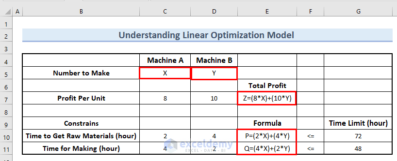
Decision Variables:
- We take X as the number of Machine A to make.
- We take Y as the number of Machine B to make.
- The question asks us to find out the maximum number of X and Y.
Note: Here, we display X and Y in the dataset so that you understand the problem. However, while performing calculations, we will get rid of these variables and will keep the cell empty.
Objective Function:
- Here, we have to maximize the Total Profit.
- Therefore, Objective function Z= (unit cost for Machine A times X)+(unit cost for Machine B times Y).
- That can be written as Z=(8*X)+(10*Y).
Constraints:
- Here, we have 2 constraints.
- For the first constraint, we can write P=(2*X)+(4*Y) in cell E10.
- And for the second contrast, we can write Q=(4*X)+(2*Y) in cell E11.
- Next, we will use the Solver tool to find out X, Y, Z, P, and Q.
Also, we will show you the actual numerical calculation in the following article.
Read More: How to Make Price Optimization Models in Excel
Step-2: Adding Solver Tool
By default, the Solver tool is not enabled in Excel. Therefore, we have to enable the Solver tool to solve the linear optimization model in Excel.
- In the beginning, we will go to the File tab.

- After that, select Options.
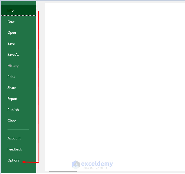
- At this point, an Add-ins dialog box will appear.
- Then, from Add-ins >> select Go.

- Then, we will mark Solver Add-ins >> click OK.

- Therefore, you can see the Solver tool in the Data tab.
Step-3: Setting Formula in Optimization Model
In this step, we will set formulas in the optimization model. We have already discussed these formulas in Step-1. Now, we will show you the actual calculation of the formulas.
- In the beginning, we will type the following formula in cell E7 to set the Objective.
=($C$5*C7)+($D$5*D7)- This formula simply makes a relation between the Number to Make and Cost Per Unit.

- After that, press ENTER.
- Since cells C5 and D5 have no values, the formula returns 0 in cell E7.
- However, after using Solver, we will get a definite value in cell E7.

- Next, we will set the formula for the Constraints.
- Afterward, we will type the following formula in cell E10.
=($C$5*C10)+($D$5*D10)- This formula simply creates a relation between the Number to Make and Time to Get Raw Materials (hour).
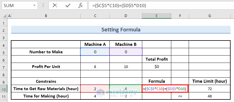
- After that, press ENTER.
- Therefore, you can see the result in cell E10.
- Further, we will drag down the formula with a Fill Handle tool.

- Therefore, you can see cells E10:E11 has 0 values in them.
- Further, we will use the Solver tool to find out the values in these cells.

Read More: How to Perform Multi-Objective Optimization with Excel Solver
Step-4: Using Solver Tool to Solve Linear Optimization Model
In this step, we will use the Solver tool to solve the linear optimization model.
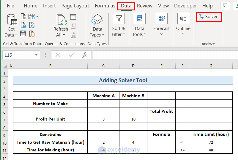
- In the first place, we will go to the Data Tab >> select Solver.

- At this point, a Solver Parameters dialog box will appear.
- Then, in the Set Objective box, we will select cell E7.
- Afterward, since we want to maximize the profit, we will select Max.
- After that, in the By Changing Variables Cells box >> we will select cells C5:D5.
- Along with that, we will click on Add.

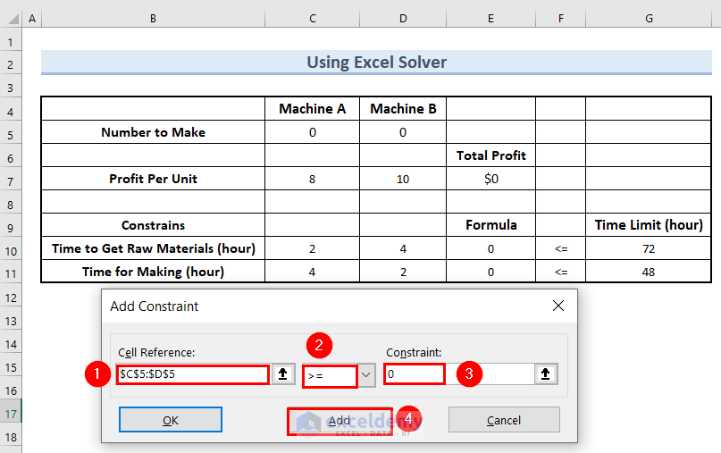
- At this moment, an Add Constraint dialog box will pop up.
- Then, select cells C5:D5 in the Cell Reference box.
- Along with that, we will select >= in the next box.
- Moreover, in the Constraint box >> select 0.
- This is because none of the variables are less than 0.
- Furthermore, click on Add.
- This will also bring an Add Constraint dialog box.
- Then, we will select cells E5:E11 in the Cell Reference box.
- Along with that, we will select <= in the next box.
- Moreover, in the Constraint box >> we will select cells G10:G11.
- Afterward, click OK.

- At this point, make sure to mark the Make Unconstrained Variables Non-Negative box.
- Furthermore, from the Select a Solving Methods >> select Simplex LP.
- Additionally, click Solve.

- Then, a Solver Results dialog box will pop up.
- Here, make sure to mark the Keep Solver Solution box.
- Then, click OK.

- Therefore, you can see the optimum Machine A number in cell C5, and the optimum Machine B number in cell D5.
- Along with that, you can see the maximum Total Profit in cell E7.

Things to Remember
- The “Solver” feature is not enabled by default. Therefore, we must enable it to perform the task.
- We must set the objective cell.
- We must set the constraints to perform the task.
Practice Section
You can download the above Excel file to practice the explained method.

Download Practice Workbook
You can download the Excel file and practice while you are reading this article.
Conclusion
Here, we tried to show you 4 easy steps for a linear optimization model in Excel. Thank you for reading this article, we hope this was helpful. If you have any queries or suggestions, please let us know in the comment section below.
Related Articles
- Solve Network Optimization Model in Excel
- Excel Optimization with Constraints
- How to Perform Route Optimization in Excel
- Schedule Optimization in Excel
- How to Optimize Multiple Variables in Excel
- How to Calculate Optimal Product Mix in Excel
- Mean Variance Optimization in Excel
<< Go Back to Optimization in Excel | Solver in Excel | Learn Excel
Get FREE Advanced Excel Exercises with Solutions!
