Mean Variance Optimization in Excel (With Easy Steps)

What Is Mean Variance Optimization?

Mean variance optimization is an analysis tool in modern portfolio theory. With the assumptions through mean variance optimization, investors can make rational investment decisions based on complete information.

Mean variance optimization is determined by the following two components:

Variance – represents how varied or spread out the numbers are in a set through numerical values based on a period of time.
Expected Return – the probability of expressing the estimated return of the investment.

When two securities have a similar return, the one with the lower variance is preferable for investment. Otherwise, investors will pick the security with the higher return while having a similar variance.

But in modern portfolio theory, an investor may differentiate his/her choice in securities with different levels of variance and expected return. The aim of this is to reduce the risk of catastrophic loss in rapidly changing market conditions.

How to Perform Mean Variance Optimization in Excel: Step-by-Step Process

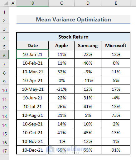
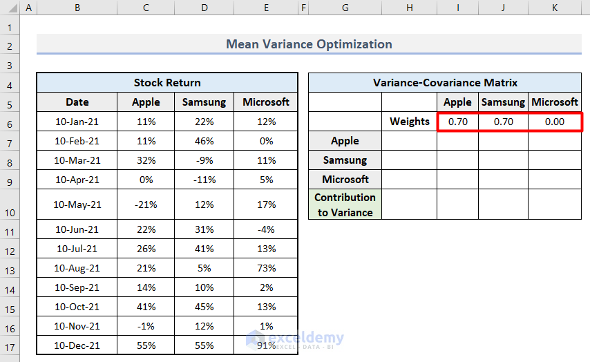
Step 1 – Prepare the Dataset

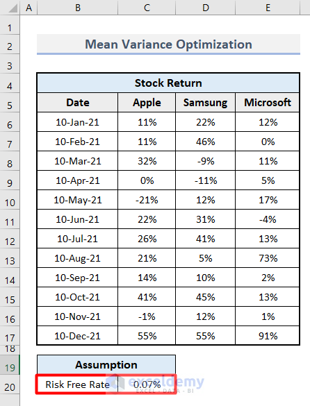
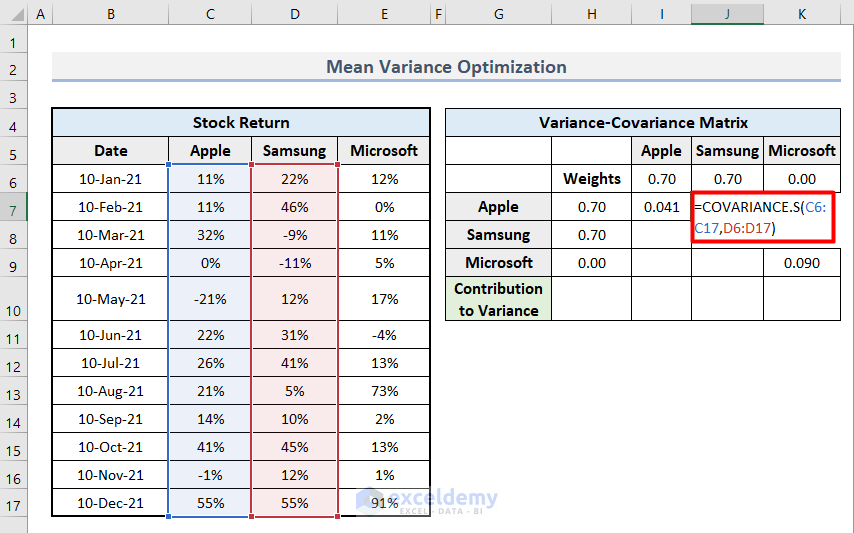
We prepared a sample dataset with the information on Stock Returns of 3 companies, Apple, Samsung, and Microsoft, in cell range B6:E17. Each of the stock returns is given within a time period of one year.

Insert the Assumption value in cell C20.

Step 2 – Calculate the Expected Return

Select cell H5 and insert this formula.

=AVERAGE(C6:C17)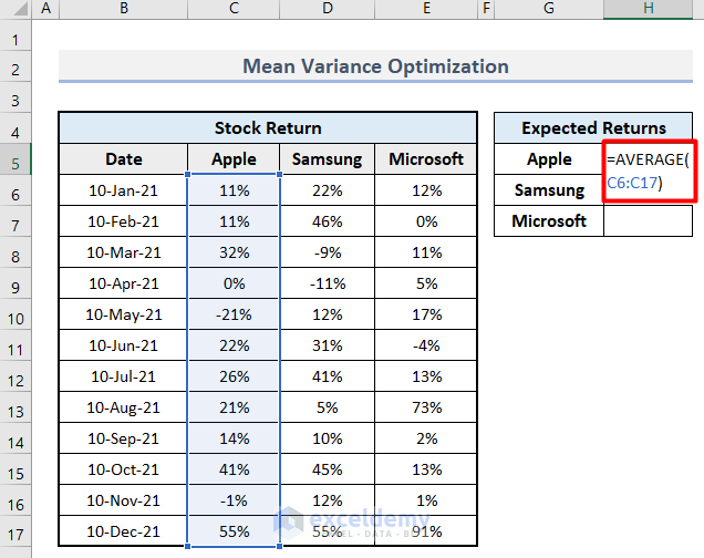

Press Enter and Autofill through the column.

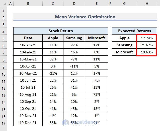
In this formula, the AVERAGE function returns the cumulative average of stock returns of each product through the selected cell range.

Format the values as percentages by selecting the range and clicking the % icon from the ribbon.

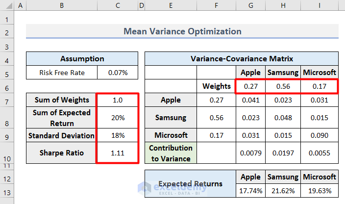
Step 3 – Make the Variance-Covariance Matrix

Determine a generic value of weights for each company. It is the percentage of investment of the companies. Insert the values as shown in the image in the cell range I6:K6.

Insert this formula as the vertical cell reference of the Weight of the company Apple and press Enter.

=I6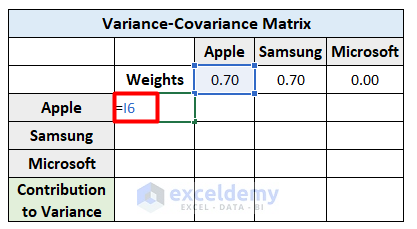

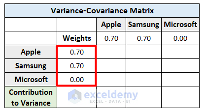
Repeat the same method to determine all the weight references in cells H8 and H9.

Select cell I7 and insert this formula to calculate the percentage of variance.

=VAR.S(C6:C17)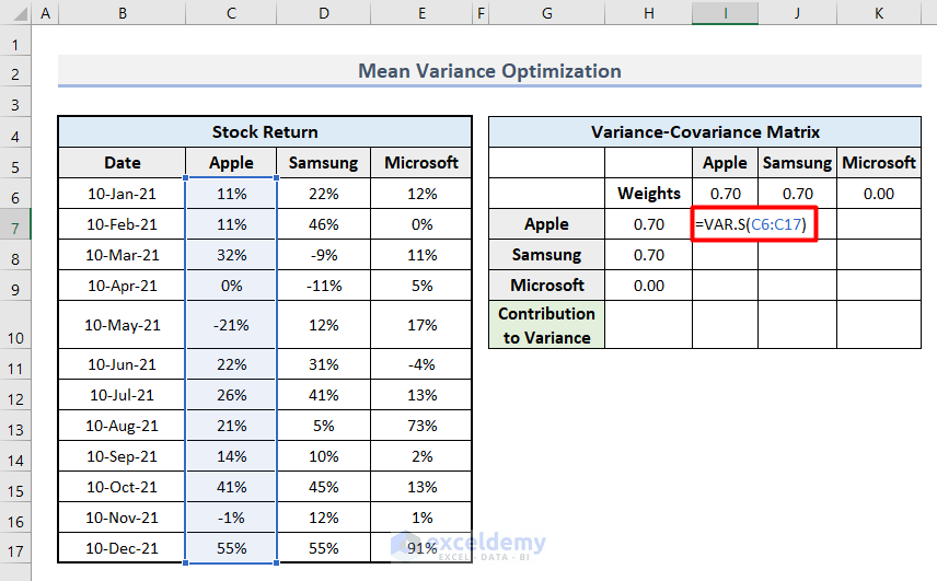

Press Enter.
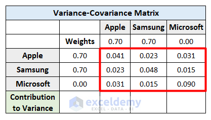
Apply the formula for each company diagonally to see the output.

We used the VAR.S function to estimate the variance based on the sample that we gave before in the Stock Return of each company.

Calculate the covariance in the rest of the cells by inserting the following formula in cell J7.

=COVARIANCE.S(C6:C17,D6:D17)

Hit Enter.

Apply the same process for each blank cell to determine the covariance of each co-existing company.

The COVARIANCE.S function returns the sample covariance and the average of the standard deviation of each pair of datasets.

Use this formula in cell I10 to get the sum of variance by each company as the contribution.

=I6*SUMPRODUCT($H$7:$H$9,I7:I9)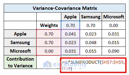

Press Enter.
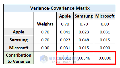
Apply the formula for each company and you will get the final output.

Here, the SUMPRODUCT function returns the sum of the variance and covariance values based on the given cell range.

Step 4 – Create the Inputs for Optimization

Calculate the Sum of Weights in cell C7 with this formula.

=SUM(G6:I6)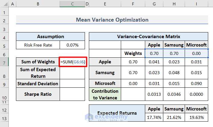

The SUM function calculates the total amount of weights of the 3 companies.

Calculate the Sum of Expected Return with this formula in cell C8.

=SUMPRODUCT(G13:I13,G6:I6)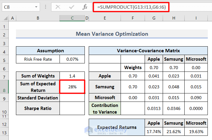

Apply the following formula in cell C9 to get the total Standard Deviation.

=SUM(G10:I10)^(1/2)

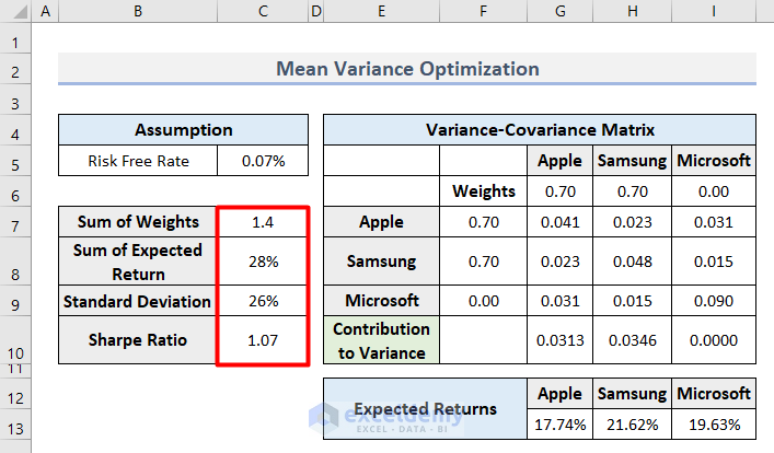
Use the following formula in cell C10 to get the expected Sharpe Ratio which compares the return of an investment with its risk.

=(C8-C5)/C9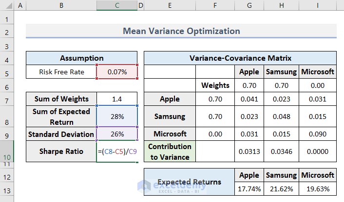

That completes the inputs.

Step 5 – Enable the Solver in the Workbook

Go to the File tab on your workbook.

Select Options from the left panel.

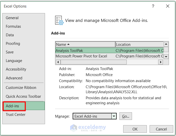
Select Add-ins in the Excel Options dialogue box.

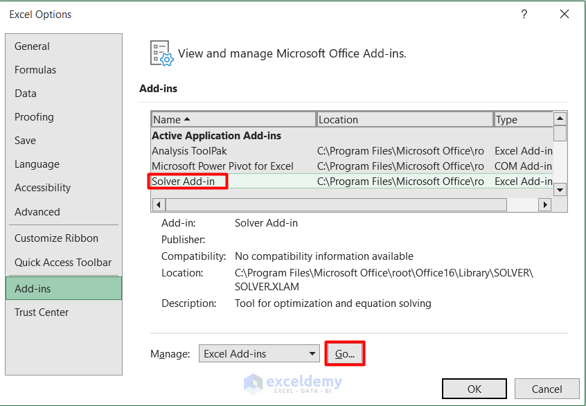
Select Solver Add-in from the Add-ins list.
Press Go.

Select Solver Add-in from the Add-ins available list.

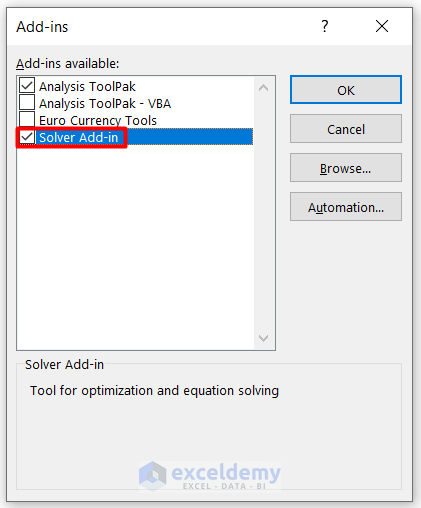
Press OK to complete the process.

Step 6 – Perform the Mean Variance Optimization

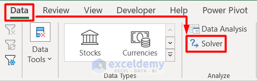
Go to the Data tab and select Solver under the Analyze group.

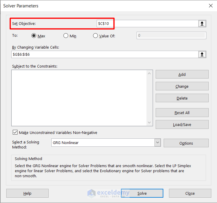
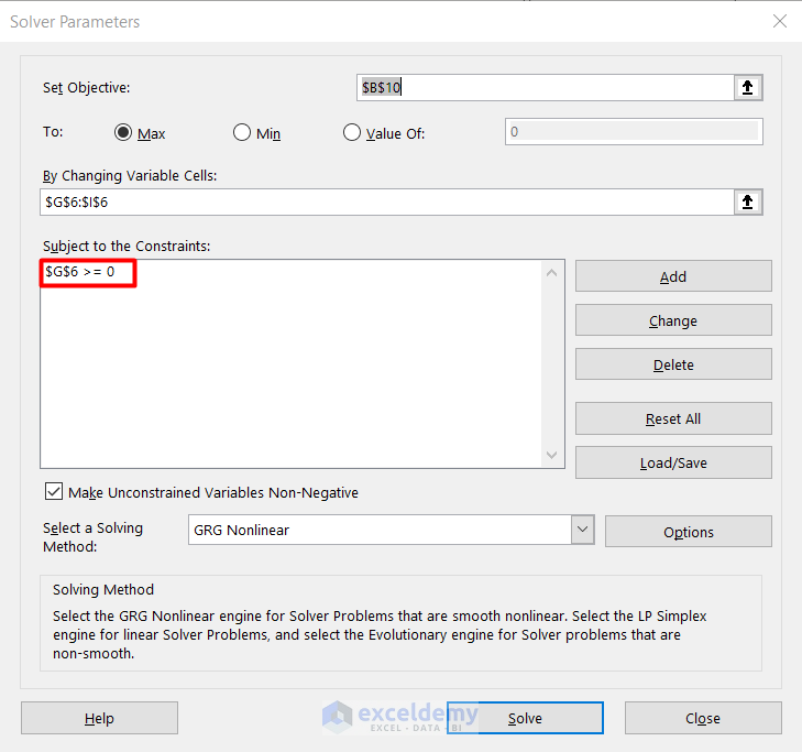
You will see the Solver Parameters dialogue box.
Insert cell C10 as an Absolute Cell Reference in the Set Objective box.

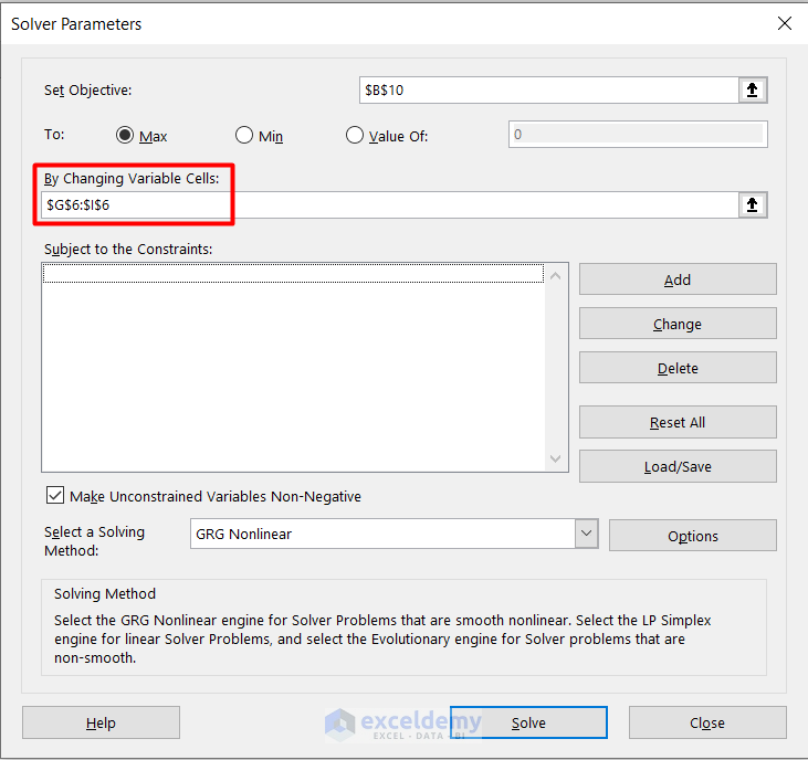
Type the cell range reference in the By Changing Variable Cells box like this.

Click on Add in the dialogue box.

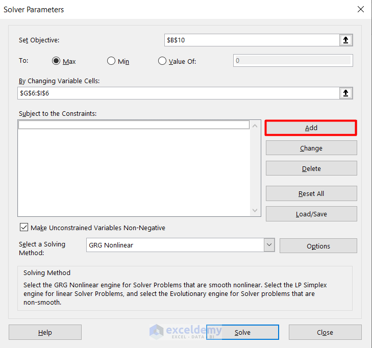
You will see the Add Constraint dialogue box.
Insert the Cell Reference and Constraint with a condition as shown in the image.

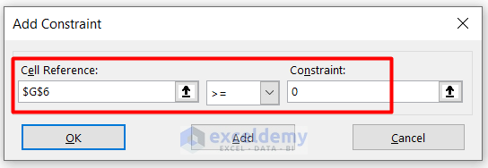
Press Add and then click on Cancel.
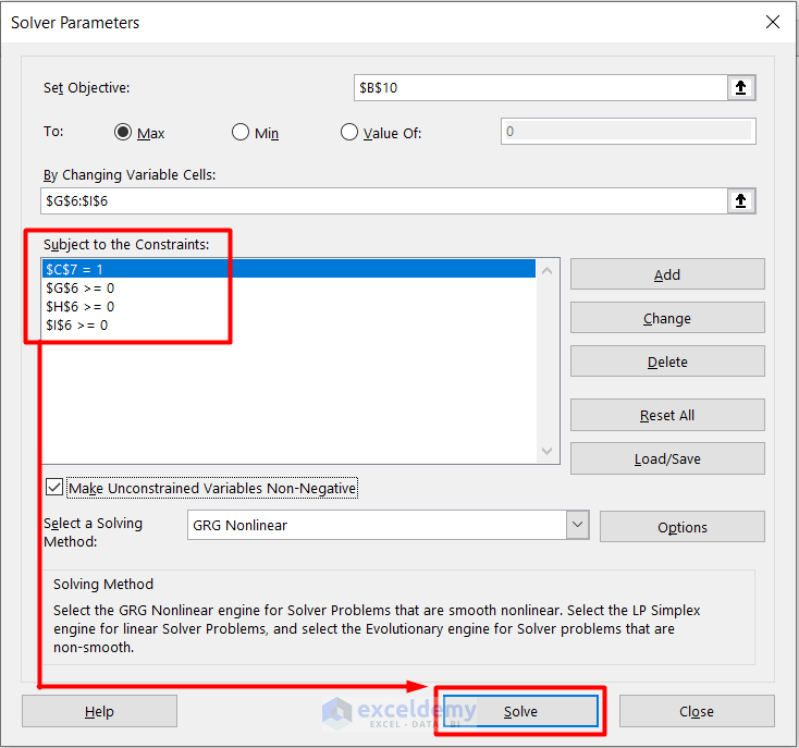
The constraint is added in the Subject to the Constraints box.

Follow the same procedure for each reference cell and click on Solve.

Note: The Sum of Weights will always be 1. This is why we put the constraint for cell C7 as $C$7 = 1.

Check the Keep Solver Solution box in the Solver Results window.
Hit OK.

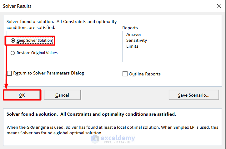
Here’s the result.

With this process, any investor will determine the risk based on the value of the expected Sharpe Ratio. It will continuously change when the Weights are changed according to market conditions.

Read More: Schedule Optimization in Excel

Limitations of the Mean Variance Optimization

The calculation of standard deviation or variance for risk is only valid for normally distributed returns. This is mostly true for traditional stocks, bonds, and derivatives.
The theory assumes that investors will not alter their asset distribution after the mean variance optimization.

Download the Practice Workbook

Mean Variance Optimization.xlsx

<< Go Back to Optimization in Excel | Solver in Excel | Learn Excel

Get FREE Advanced Excel Exercises with Solutions!