How to Use VAR Function in Excel (4 Examples)

The Excel VAR function is categorized as a Statistical function of Microsoft Excel. It determines the risk of any investment, hence, is important for financial organizations. In this article, we will discuss the use of the Excel VAR function with examples and proper illustration.

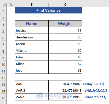
From the above image, you will get a brief idea of getting the variance of a data set.

Download Practice Workbook

Download this practice workbook to exercise while you are reading this article.

Introduction to VAR Function

Function Objective:

The VAR function returns the variance of a sample taken from population data.

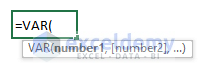
Syntax:

VAR(number1,[number2],…)

Argument:

Return Parameter:

It returns a numeric value.

Available in:

Excel for Microsoft 365, Microsoft 365 for Mac, Excel for the web Excel 2021, Excel 2021 for Mac, Excel 2019, Excel 2019 for Mac, Excel 2016, Excel 2016 for Mac, Excel 2013, Excel 2010, Excel 2007, Excel for Mac 2011, Excel Starter 2010

Note:

This function has been replaced by one or more new Excel functions. Those functions may provide better accuracy. Still, this function is available for the older version’s compatibility. But we should practice using the new functions as well, because this function may not be available in future versions according to support.microsoft.com.

Different VAR Functions in Excel

We have multiple VAR functions according to their usages in Microsoft Excel. They are as below:

Note:

The VAR function is now modified to VAR.S and used in the latest versions of Microsoft Excel. We can use VAR.S instead of VAR and get the same result.

What is Variance?

Variance is the amount of variability of the data set, which indicates how different is spread among values. Mathematically, it is the average of the square values of the difference. The basic formula for calculating variance is as follows:

Here,

x = Sample values, A= Mean or the average of the sample values, n = Number of sample values.

How to Use the VAR Function in Excel

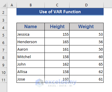
Now, we will show how to use this Excel VAR function. We have taken data of some students with their height and weight. Now, we will calculate the variance of the height of the students here.

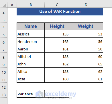
Step 1:

• Add a box for the Variance.

Step 2:

• Now, type the VAR function.
• The formula will be:

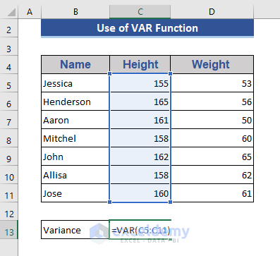
Step 3:

• Now, press Enter.

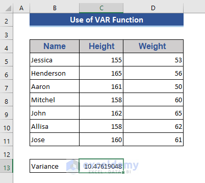
We get the variance here.

Crosscheck the Result from VAR Function with a Manual Procedure: 

We can crosscheck and show the calculation manually.

Step 1:

• First, find the mean of the range using the AVERAGE function.

Step 2:

• Now, subtract the mean value from each of the sample values. Apply the following formula:

• Put formula for the next cells in the same way.

Step 3:

• Now, calculate the square of each difference using the below formula.

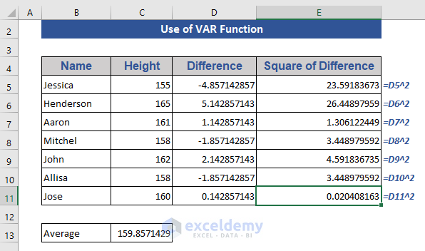
Step 4:

• Now, we will find out the variance by applying the following formula:

Step 5:

• Then press Enter.

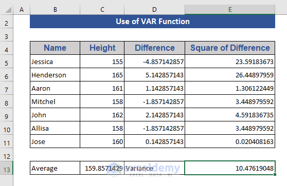
The final output is the same we’ve got using the VAR function first.

Read More: How to Use COUNTA Function in Excel (3 Suitable Examples)

4 Examples of Using VAR Function in Excel

We can use the VAR function in different ways. We will show the use of this function with the following examples. Let’s see one by one.

1. Find Out Variance of Individual Numbers Using VAR Function

In this example, we will insert individual numbers in the formula. We will consider the below data for this example.

Let’s see the steps below.

Step 1:

• Go to Cell C13.
• Write the VAR function and input the data individually.
• So, the function will become-

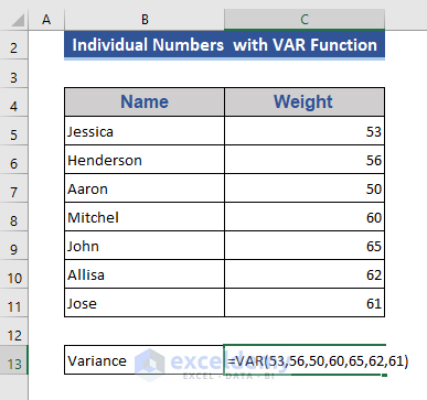
Step 2:

• Then press Enter.

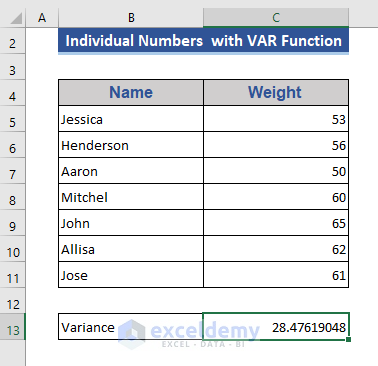
This is the required variance.

2. Get Variance of a Single Range Using VAR Function

Here, we will get the variance of a single range applying the VAR Function. We have only a single range in our data set.

Let’s go through the following steps.

Step 1:

• We will insert a range in the VAR function.
• So, the formula will be-

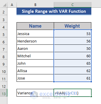
Step 2:

• Then press Enter.

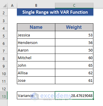
Here, we get the variance of a single range.

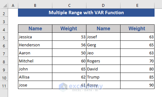
3. Apply Excel VAR Function with Multiple Ranges

This example shows the use of the VAR function with multiple ranges of data. If we need to find variance from different columns, then we will apply this way.

We have taken the below data for this example.

Now, see the following steps.

Step 1:

• Now, write the VAR function.
• Input both ranges using a comma between them.
• So, the formula is:

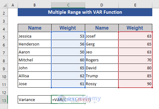
Step 2:

• Then, press Enter.

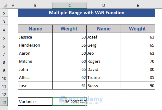
Here, we show when we have multiple ranges of data then how we will apply the VAR function.

4. Number Arrays with VAR Function

We can also use an array of numbers with the VAR function. In this example, we insert an array together with a range. See how we do this in the following manner.

Step 1:

• Type the formula in Cell C13:

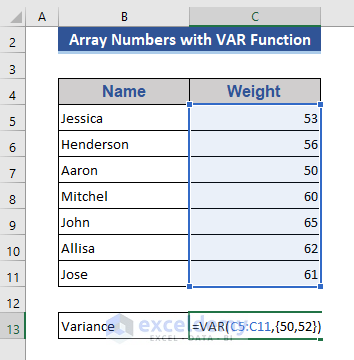
Step 2:

• Now, press Enter.

We get the variance using the array of numbers.

Similar Readings

• How to Use RANK Function in Excel (With 5 Examples)
• Find Mean Median and Mode on Excel(4 Easy ways)
• How to Use MODE Function in Excel (4 Examples)
• Use PROB Function in Excel (3 Examples)
• How to Use Excel STDEV Function (3 Easy Examples)

Use of Other VAR Functions to Calculate Variance

1. VAR.S Function as a Counterpart of VAR Function

The VAR.S Function does the same operation as the VAR function. The VAR.S function is available in Excel 2010 and later versions.

The arguments of VAR.S are also the same as the VAR function.

We can show that the return of VAR and VAR.S functions are the same from the below image.

We have just typed the following formulas.

Type the following formula in Cell C13-

Enter the formula in Cell C14-

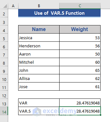
2. VARA Function That Considers Boolean Logics and Text Values

The VARA function is a bit different from the VAR and VAR.S functions. The VAR and VAR.S functions ignore the Boolean and Text values. But the VARA function evaluates the text as 0, FALSE as 0, and TRUE as 1. So, it is important to carefully choose the suitable Excel function when we calculate the variance.

The VARA function is like this:

For this example, we’ve taken the following dataset where text value exists.

Now, we’ll show the difference between the VARA function with the VAR and VAR.S function.

Apply VAR, VAR.S, and VARA functions in Cell C13, C14, and C15.

Enter the following formula in Cell C13.

The formula in Cell C14 will be-

The formula in Cell C15 is-

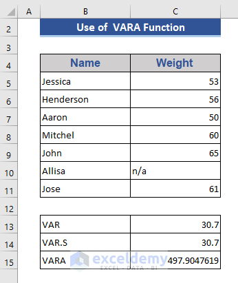
Here, we can see that from VAR and VAR.S, we get the same result. But the VARA returns a different result from them. Because the VARA function counts the text values as 0.

Read More: How to Use COUNT Function in Excel (With 5 Examples)

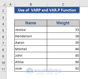
3. Use of VARP and VAR.P to Calculate Population Variance

VARP and VAR.P are the same functions. The VARP is applicable for Excel 2000 to 2019 and VAR.P is applicable for Excel 2010 to later versions. Both functions are used to get population variance. It means how data in the entire population is spread out. The mathematical formula for population variance is:

Here,

x = Sample values, A= Mean or the average of the sample values, n = Number of sample values.

Now, we will find out the population variance of the below data.

Step 1:

• Write the VARP function in Cell C13.
• Now, the complete formula will be-

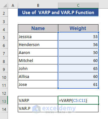
Step 2:

• Now, press Enter.

Step 3:

• Now, we will apply the VAR.P function on Cell C14.
• The complete formula is:

Step 4:

• Again, press Enter.

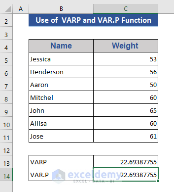
Here, we showed the use and result of the VARP and VAR.P function

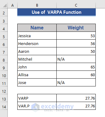
4. VARPA Function That Considers Boolean Logics and Text Values

The VARPA and VARP and VAR.P do the same operation. But VARP and VAR.P ignore the texts and boolean logic. On the other hand, the VARPA evaluates the text as 0, TRUE as 1, and FALSE as 0, and hence gives a different result.

Assume that some students’ weight is not available. So, the data set will look like this:

Step 1:

• Now, get the VARP and VAR.P by applying the following formulas in Cell C13 and Cell C14.
• Formula in Cell C13 is:

• The formula in Cell C14 is:

Step 2:

• Now, we will get the VARPA in the same way in Cell C15.

Here, we get population variance for different population functions that exist in Excel.

Read More: How to Use Different Types of COUNT Function in Excel(5 Ways)

Things to Remember

• When the function contains less than 2 numeric values error will occur, that error is #DIV/0!.
• If any text value is supplied to the function, it will show an error.
• In case we use the entire population, then we must apply VARP to compute the variance.
• If we include logical values and texts in the function argument, then we must use the VARA function to calculate variance.

Conclusion

In this article, we showed the use of the VAR function in Excel with suitable examples. I hope this will satisfy your needs. Please have a look at our website Exceldemy.com and give your suggestions in the comment box.

Related Articles

• How to Use Excel GROWTH Function (4 Easy Methods)
• Use TREND Function in Excel (3 Examples)
• How to Use Excel NORMDIST Function (2 Applications)
• Use INTERCEPT Function in Excel
• How to Use NORMINV Function in Excel
• Use QUARTILE Function in Excel (5 Suitable Examples)