Unquestionably, Microsoft Excel excels at crunching numbers! Now, this means that you can perform network optimization in the blink of an eye. In this regard, Excel becomes a convenient and valuable tool. Granted this, this article demonstrates 3 cases of how to solve network optimization model in Excel. In addition, we’ll also explore how to solve schedule optimization in Excel.
How to Solve Network Optimization Model in Excel: 3 Cases
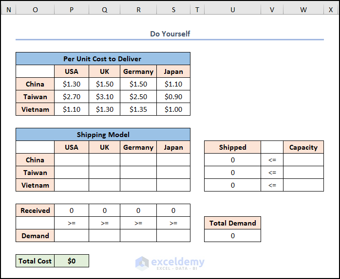
In the first place, let’s familiarize ourselves with the dataset shown in the image below, where we have the “Per Unit Cost to Deliver” array in the B5:F8 cells, the maximum “Capacity” of the suppliers “China”, “Taiwan” and “Vietnam”, and the maximum “Demand” of the consumers “USA”, “UK”, “Germany” and “Japan” respectively. Here, we want to solve the network optimization model in Excel with the use of the Solver Add-in. In the following sections, we’ll learn more about each of the cases in detail and with the necessary illustrations.
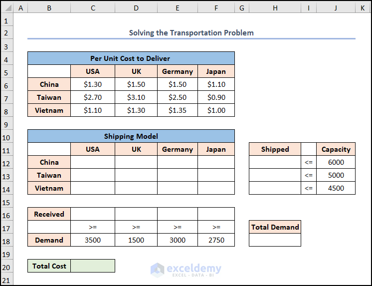
Here, we have used the Microsoft Excel 365 version; you may use any other version according to your convenience.
1. Solving Transportation Problem
First and foremost, let’s start with a simple case of the network optimization model where we’ll solve the transportation problem. In this scenario, we’ll optimize various constraints to obtain the minimum cost of transport. Here, we’ll use the SUM and SUMPRODUCT functions to calculate the sum of an array and return its product.
📌 Steps:
- First, click the File tab >> go to Options.
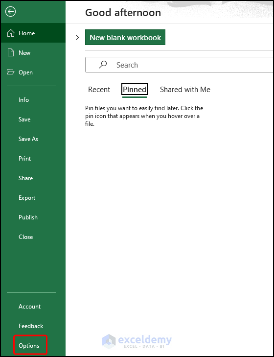
- Next, select Add-ins >> choose Excel Add-ins >> press the Go button.

- Then, click on the Solver Add-in >> hit the OK button to activate the Solver program.

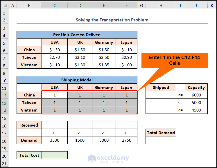
- Second, select the C12:F14 cells >> enter the value “1” as the initial value.
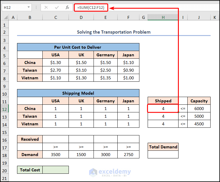
- Following this, move to the H12 cell >> enter the formula given below >> use the Fill Handle tool to copy the formula into the cells below.
=SUM(C12:F12)
Here, the C12:F12 range refers to the “USA”, “UK”, “Germany” and “Japan” values corresponding to “China”.
- Afterward, navigate to the C16 cell >> insert the following expression >> copy the formula across up to the F16 cell.
=SUM(C12:C14)
For instance, the C12:C14 cells represent the “China”, “Taiwan” and “Vietnam” values that correspond to “USA”.

- In turn, apply the equation in the H18 cell to get the “Total Demand”.
=SUM(C18:F18)
On this occasion, the C18:F18 array indicates the “Demand” of each of the consumers.

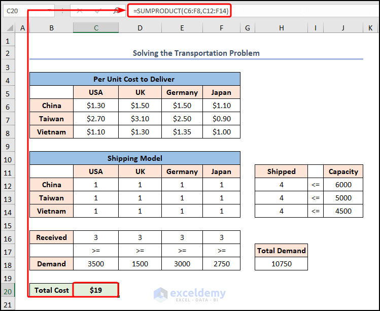
- Later, enter the C20 cell to copy and paste the formula given below.
=SUMPRODUCT(C6:F8,C12:F14)
Formula Breakdown:
- SUMPRODUCT(C6:F8,C12:F14) → returns the sum of the products of the corresponding ranges or arrays. Here, the C6:F8 and C12:F14 are the array1 and array2 arguments which are multiplied and added together to return the output.
- Output → $19
- Third, jump to the Data tab >> press the Solver icon.
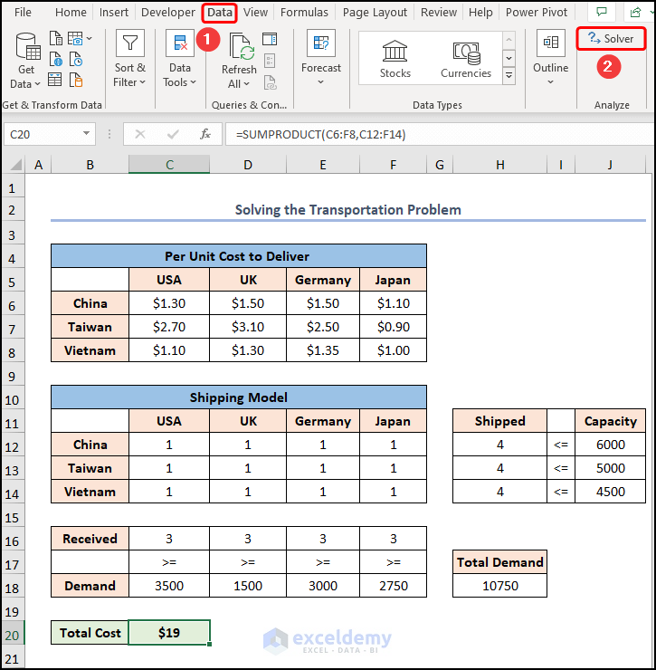
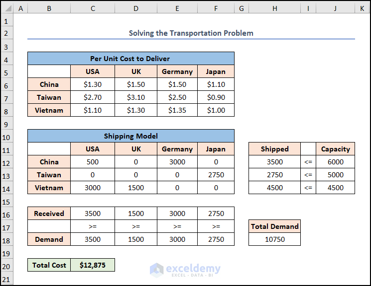
Finally, the results should look like the screenshot shown below.
Read More: How to Solve Linear Optimization Model in Excel
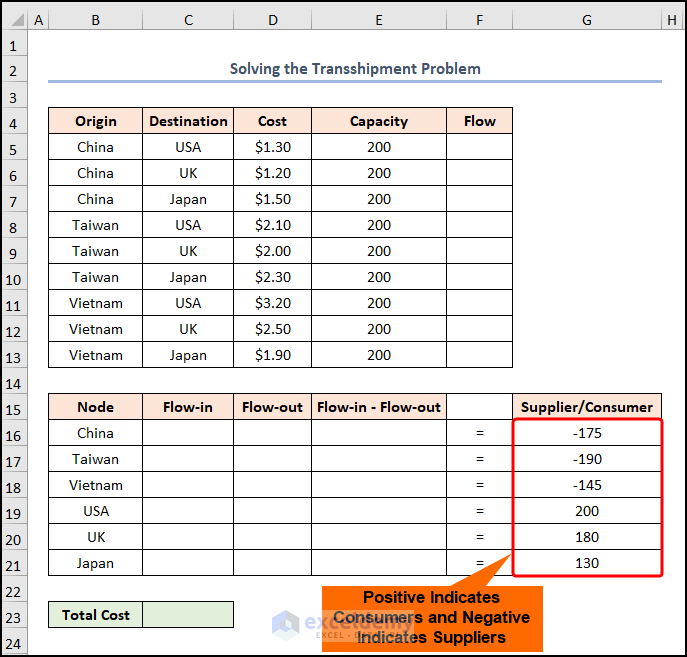
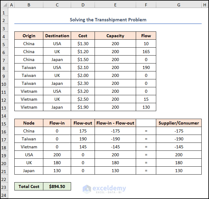
2. Evaluating Transshipment Problem
Alternatively, the next case of the network optimization model considers the transshipment problem, where we ship goods from the “Supplier” to the “Consumer” while ensuring the least cost. Moreover, in this scenario, all the “Suppliers” have a fixed “Capacity” of “200”. Here, we’ll utilize the SUMIF function to add up the cells which fulfill certain criteria.
📌 Steps:
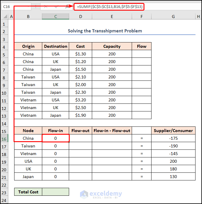
=SUMIF($C$5:$C$13,B16,$F$5:$F$13)
Formula Breakdown:
- SUMIF($C$5:$C$13,B16,$F$5:$F$13) → adds the cells specified by a given criteria or condition. Here, C5:C13 is the range argument that refers to the “Destination” column. Then, B16 represents the criteria argument (“China”) to apply within the given range. Lastly, F5:F13 is the optional sum_range argument which indicates the “Flow” values to sum within the range.
- Output → 0
📃 Note: Please make sure to use Absolute Cell Reference by pressing the F4 key on your keyboard.
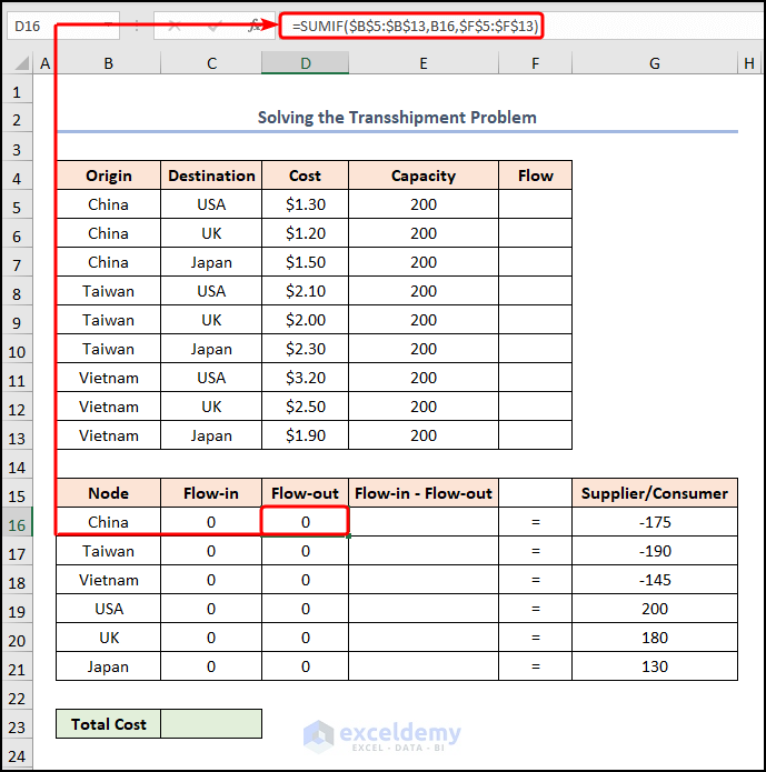
- In a similar style, apply the expression below to the D16 cell.
=SUMIF($B$5:$B$13,B16,$F$5:$F$13)
For example, the B5:B13 and F5:F13 cells point to the “Origin” and “Flow” columns respectively.
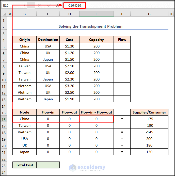
- Then, obtain the difference between the in-flow and out-flow values as shown below
=C16-D16
Here, the C16 and D16 cells refer to the in-flow and out-flow values for “China”.
- Next, compute the “Total Cost” by applying the equation below.
=SUMPRODUCT(F5:F13,D5:D13)
In this situation, the F5:F13 and D5:D13 arrays represent the “Flow” and “Cost” columns.

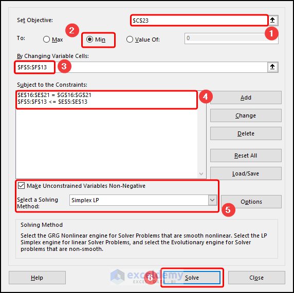
- Eventually, choose the options shown in the picture below or follow the prior steps to run the Solver.
Consequently, the final output should appear in the figure below.
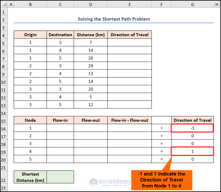
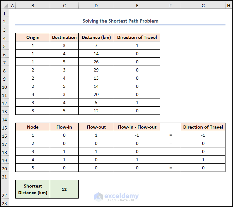
3. Solution of Shortest Path Problem
For one thing, another case of the network optimization model problem requires solving for the shortest path between two points using the Solver Add-in in Excel. In this case, we want to calculate the shortest distance between “Node 1” and “Node 4” so we’ve entered “-1” and “1” to indicate the “Direction of Travel” from “Node 1” to “Node 4”.
📌 Steps:
- Initially, follow the steps shown in the previous method to compute the “Flow-in”, “Flow-out” and the “Flow-in – Flow-out”.
- Afterward, go to the C22 cell >> type in the formula given below.
=SUMPRODUCT(E5:E13,D5:D13)
For instance, the E5:E13 and D5:D13 range of cells point to the “Direction of Travel” and “Distance (km)” columns.

- Likewise, choose the options shown below in the Solver window.
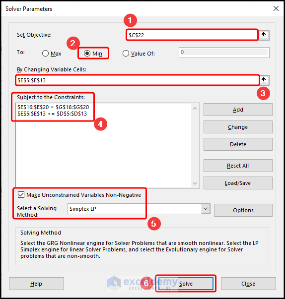
Subsequently, completing the above steps yields the results shown in the image below.
Read More: How to Perform Route Optimization in Excel
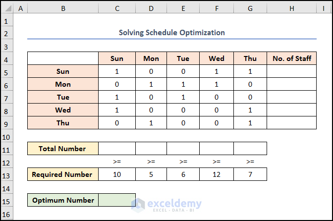
How to Solve Schedule Optimization in Excel
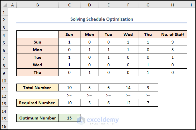
Last but not least, we can make a Work Schedule to make sure the optimum number of staff is present throughout the week to maintain a smooth operation. For instance, the “1” represent a workday in contrast “0” refers to an off day.
📌 Steps:
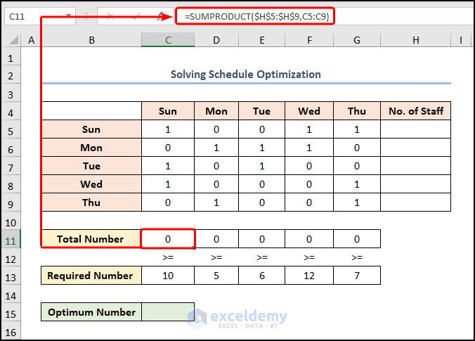
- First and foremost, enter the C11 cell to insert the formula given below.
=SUMPRODUCT($H$5:$H$9,C5:C9)
In this case, the H5:H9 and C5:C9 arrays indicate the “No. of Staff” and the “Sun” columns
- In turn, calculate the “Optimum Number” using the following equation.
=SUM($H$5:$H$9)

- Later, apply the steps shown in real-time in the GIF below to solve in Excel Solver.
Lastly, the results appear in the picture below.
Admittedly, we’ve skipped some relevant examples of Schedule Optimization which you may explore if you wish.
Practice Section
We have provided a Practice section on the right side of each sheet so you can practice yourself. Please make sure to do it by yourself.
Download Practice Workbook
Conclusion
In short, this tutorial explores 3 cases of how to solve network optimization model in Excel. Now, we hope all the methods mentioned above will prompt you to apply them in your Excel spreadsheets more effectively. Furthermore, if you have any questions or feedback, please let me know in the comment section.
Related Articles
- Excel Optimization with Constraints
- How to Make Price Optimization Models in Excel
- Schedule Optimization in Excel
- How to Perform Multi-Objective Optimization with Excel Solver
- How to Optimize Multiple Variables in Excel
- How to Calculate Optimal Product Mix in Excel
- Mean Variance Optimization in Excel
<< Go Back to Optimization in Excel | Solver in Excel | Learn Excel
Get FREE Advanced Excel Exercises with Solutions!
