For illustration, let’s suppose a machine is used to produce two interchangeable products. The daily production capacity of the machine is 20 units of product 1 and 10 units of product 2. Alternatively, the machine can be adjusted to produce at most 12 units of product 1 and 25 units of product 2 daily. Market analysis shows that the maximum daily demand for the two products combined is 35 units. Given that the unit profits for the two respective products are $10 and $12, which of the two machine settings should be selected?
STEP 1: Analyze Question and Create Dataset
- Understand the given integer linear programming problem and analyze it.
- Analyzing the above question, we have the findings below.
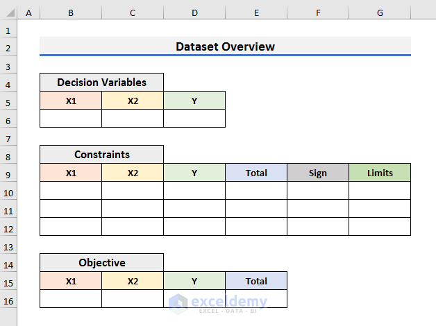
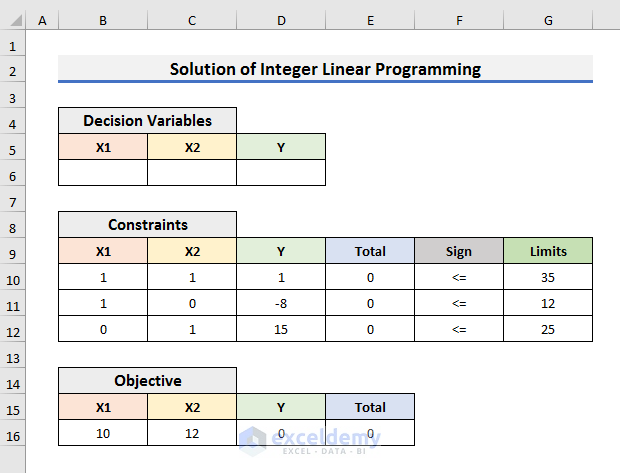
Decision Variables:
- X1: Production quantity of product 1.
- X2: Production quantity of product 2.
- Y: 1 if the first setting is selected or 0 if the second setting is selected.
Objective Function:
The objective function is:
Z=10X1+12X2
Constraints:
We can find 3 constraints from the above question. They are:
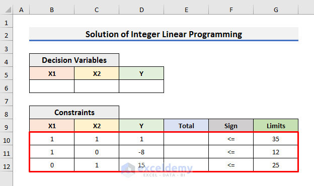
- X1+X2<=35
Because the market analysis shows that the maximum daily demand for the two products combined is 35 units.
- X1-8Y<=12
This constraint is specific for product 1.
- X2+15Y<=25
It is the constraint for the second product.
- Y={0,1}
The value of Y will be 0 or 1.
- X1,X2>=0
The quantity of the products cannot be negative.
- We have created a dataset like the image below keeping the constraints, functions and variables. You can create it according to your needs.
Read More: How to Do Linear Programming in Excel
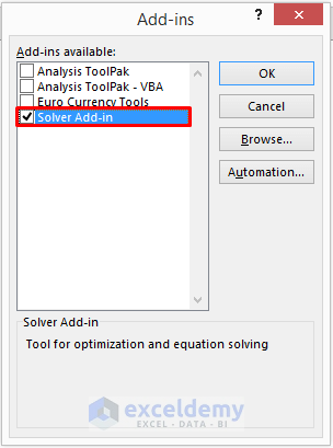
STEP 2: Load Solver Add-in in Excel
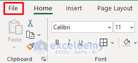
- Load the Solver add-in in Excel by clicking on the File tab.
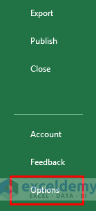
- Select Options from the left–bottom corner of the screen.
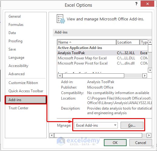
- It will open the Excel Options window.
- Select Add-ins.
- Select Excel Add-ins and click on Go in the Manage box.
- An Add-ins message box will pop up.
- Check Solver Add-in and click OK.
- The Solver feature in the Analysis section of the Data tab is loaded.
Read More: How to Solve Blending Linear Programming Problem with Excel Solver
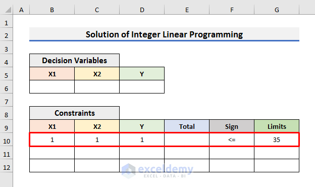
STEP 3: Fill Coefficients of Constraints and Objective Function
- Fill the constraints and objective function in the dataset.
- Insert the coefficients of the constraints and objective function.
- Our first Constraint is that X1+X2<=35. It means if the first setting is selected, the sum of the products should be equal to or less than 35.
- The coefficient of X1 is 1 and X2 is 2.
- The equation indicates the first setting, so the coefficient of Y is 1.
- The sign is <=.
- And the limit is 35.
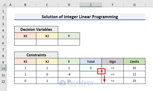
- Repeat the steps and fill in the coefficients of all the constraints.
- Select Cell E10 and enter the following formula:
=SUMPRODUCT($B$6:$D$6,B10:D10)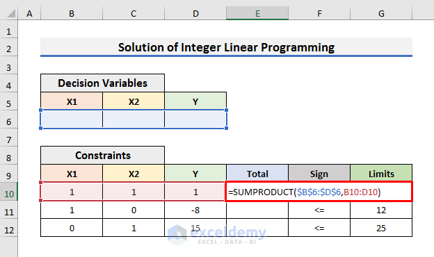
In this formula, we have used the SUMPRODUCT function to calculate the product of decision variables with the respected constraints variables and then add them up. In this case, Cell B6 will be multiplied by Cell B10, Cell C6 by Cell C10, and Cell D6 by Cell D10. All the products will be added together.
- Hit Enter and drag the Fill Handle down.
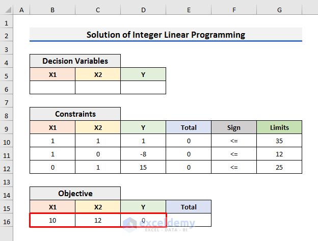
- Fill the coefficients of the objective function in Cell B16 to C16.
- In our case, the objective function is Z = 10X1+12X2.
- Select Cell E16 and enter the following formula:
=SUMPRODUCT($B$6:$D$6,B16:D16)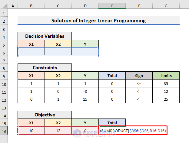
- Press Enter and the coefficients and formulas will be entered.
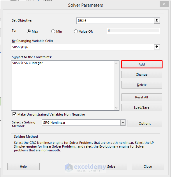
STEP 4: Insert Solver Parameters
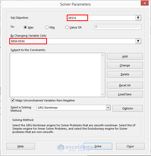
- Go to the Data From the Analyze section, select Solver. It will open the Solver Parameters window.

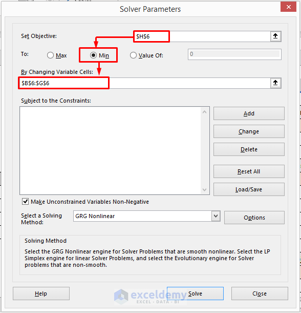
- In the Set Objective box, you need to enter the cell that will contain the value of the objective function.
- We have entered $E$16.
- We are trying to find the maximum result, so we selected Max.
- In the ‘By Changing Variable Cells’ enter $B$6:$D$6. It contains the decision variables.
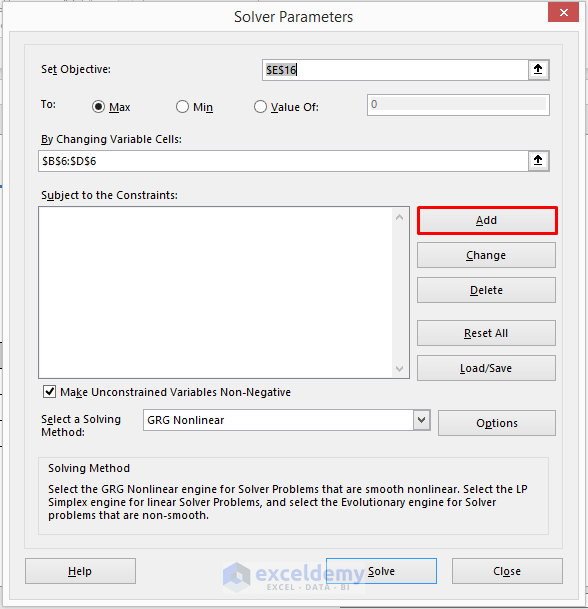
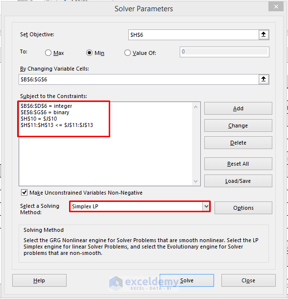
STEP 5: Add Subject to Constraints
- Add subjects to the constraints.
- We need to denote the type of variables, whether they are binary or integer and the relation of the constraints.
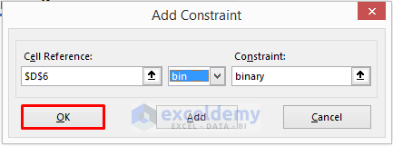
- Click on Add. It will open the Add Constraint dialog box.
- Enter $D$6 in the Cell Reference box and select bin from the drop-down menu.
- Cell D6 holds the value of Y which is 0 or 1. That indicates binary numbers. That is why we have selected the bin.
- Click OK.
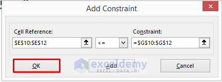
- Click on Add.
- Enter $E$10:$E$12 in the Cell Reference box, <= symbol from the drop-down menu and =$G$10:$G$12 in the Constraint box.
- Click OK.
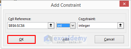
- Click Add in the Solver Parameters window.
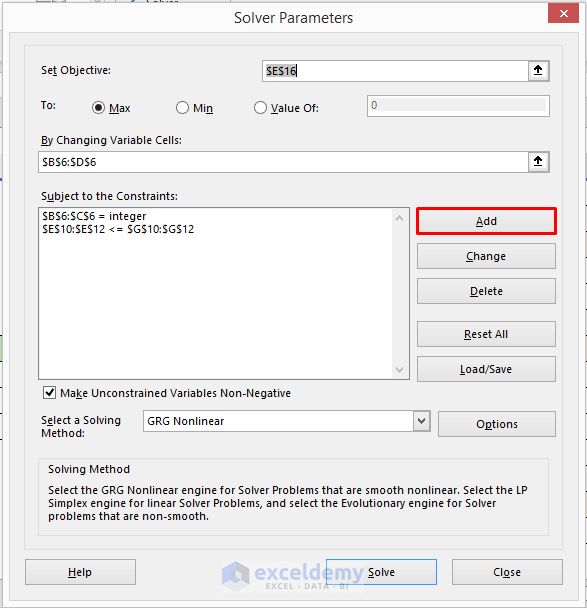
- Enter $B$6:$C$6 in the Cell Reference box and select int from the drop-down menu.
- Cell B6 and C6 store the values of X1 and X2 which are integers.
- Click OK.
STEP 6: Select Solving Method
- Select Simplex LP in the ‘Select a Solving Method’ section and click on Solve.
- Tick ‘Make Unconstrained Variables Non-Negative’.
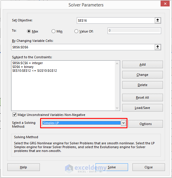
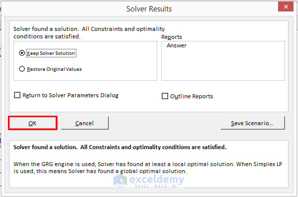
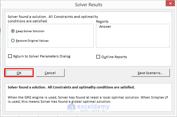
- Click on Solve and the Solver Results window opens.
- Select OK.
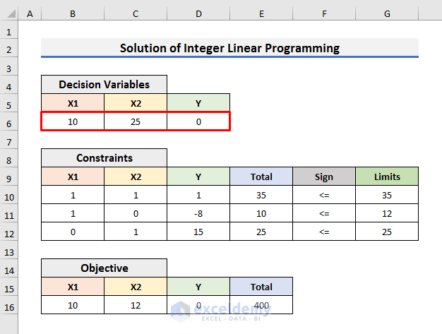
STEP 7: Solution of Integer Linear Programming
- You will find the solutions in your desired cells on the excel sheet.
- The second machine setting will provide us with the best output.
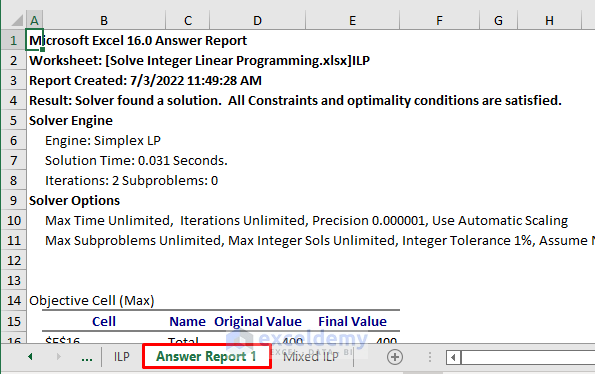
STEP 8: Generate Answer Report
- Generate the answer report.
- Select Answer in the Reports section of the Solver Results window and click OK.
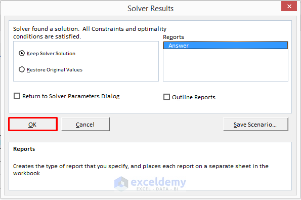
- You will get the report on a new sheet.
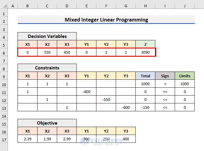
Mixed Integer Linear Programming Example in Excel
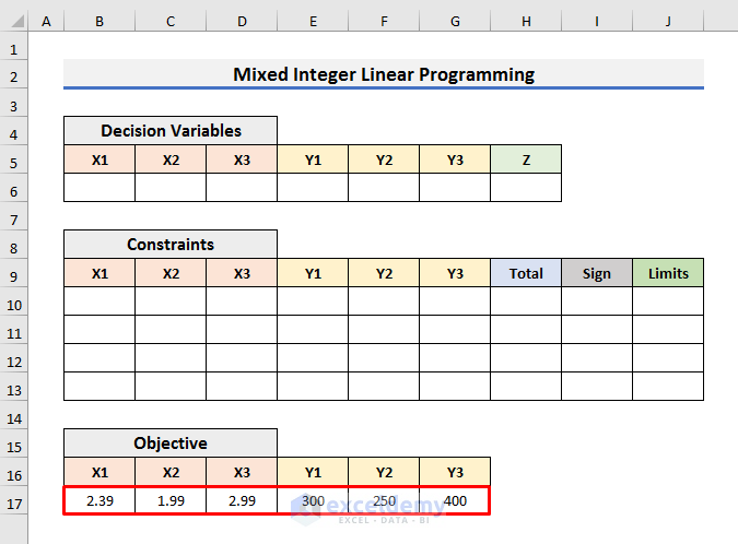
Objective Function:
Z=2.39X1+1.99X2+2.99X3+300Y1+250Y2+400Y3
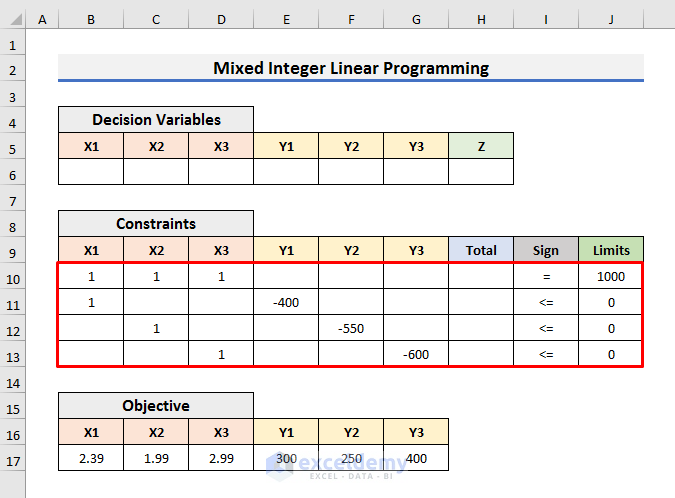
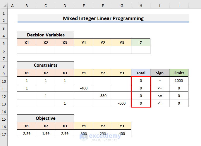
Constraints:
- X1+X2+X3=1000
- X1-400Y1<=0
- X2-550Y2<=0
- X3-600Y3<=0
X1, X2, and X3 are integers. Y1, Y2, and Y3 are binary numbers. And, we need to find the minimum value of Z.
STEPS:
- Create a dataset to store the coefficients of Decision Variables, Constraints and Objective Function.
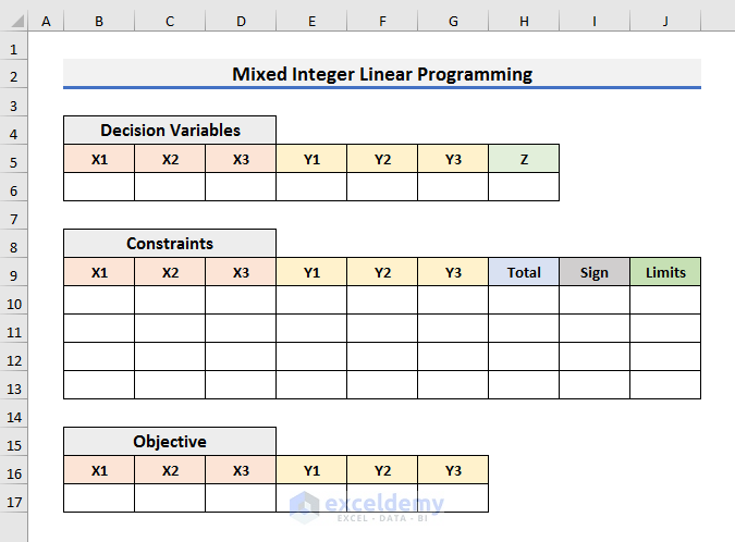
- Enter mixed coefficients of the variables of the Objective Function.
- Enter the coefficients of the variables of Constraints. Keep the Total column empty.
- Select Cell H10 and enter the following formula:
=SUMPRODUCT($B$6:$G$6,B10:G10)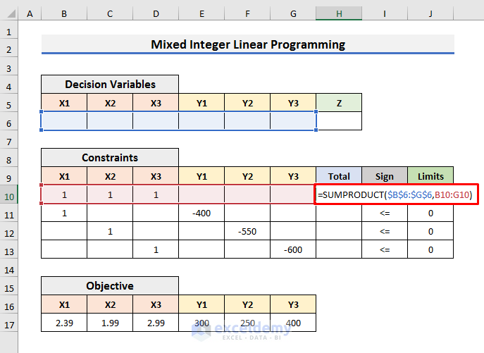
- Press Enter and drag the Fill Handle down.
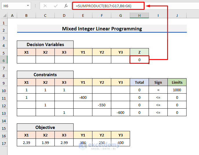
- Enter the formula below in Cell H6:
=SUMPRODUCT($B$6:$G$6,B10:G10)- Hit Enter.
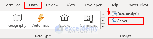
- Go to the Data tab and select Solver. It will open the Solver Parameters window.
- Set the objective at Cell $H$6 to Min by changing variable cells $B$6:$G$6.
- Click on Add.
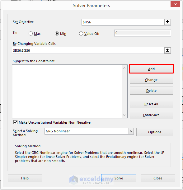
- Add the Constraints one by one and choose Simplex LP as the Solving Method.
- Click on Solve.
- The Solver Results window will open.
- Click OK.
- It will output the results.
Read More: How to Perform Mixed Integer Linear Programming in Excel
Download Practice Book
Related Articles
- How to Calculate Shadow Price Linear Programming in Excel
- Graph Linear Programming in Excel
- How to Find Optimal Solution with Linear Programming in Excel
- How to Do Linear Programming with Sensitivity Analysis in Excel
<< Go Back to Excel Linear Programming | Solver in Excel | Learn Excel
Get FREE Advanced Excel Exercises with Solutions!

Hi Mursalin. Could you please explain how you got the constraint equations?
Hi KIM,
Thanks for your comment. To explain the step-by-step solution, we used the following question here.
“Suppose, a machine is used to produce two interchangeable products. The daily capacity of the machine can produce at most 20 units of product 1 and 10 units of product 2. Alternatively, the machine can be adjusted to produce at most 12 units of product 1 and 25 units of product 2 daily. Market analysis shows that the maximum daily demand for the two products combined is 35 units. Given that the unit profits for the two respective products are $10 and $12, which of the two machine settings should be selected?”
This question is also stated before starting STEP 1.
Analyzing the above question, we can find the following constraints:
Constraint 1:
X1+X2<=35
Because the maximum daily demand for the two products combined is 35 units.
Here, X1 is the quantity of Product 1 and X2 is the quantity of Product 2.
Constraint 2:
X1-8Y<=12
This constraint is for Product 1. In this constraint, we have combined the conditions for both settings for Product 1. In setting 1, product 1 can be produced at most 20 units; in setting 2, product 2 can be produced at most 12 units.
Here, Y denotes which setting is selected. If setting 1 is selected, then Y will be 1 and if setting 2 is selected, then Y will be 0.
For example, if setting 1 is selected, then we can set Y=1. So, the equation will be:
X1-8.1<=12
As a result, the simplified constraint will be X1<=20 which clearly states the condition for product 1 stated in the first setting.
Constraint 3:
X2+15Y<=25
This constraint is for Product 2. In this constraint, we have combined the conditions for both settings for Product 2. In setting 1, product 2 can be produced at most 10 units; in setting 2, product 2 can be produced at most 25 units.
Here, Y denotes which setting is selected. If setting 1 is selected, then Y will be 1 and if setting 2 is selected, then Y will be 0.
For example, if setting 1 is selected, then we can set Y=1. So, the equation will be:
X2+15.1<=25
As a result, the simplified constraint will be X2<=10 which clearly states the condition for product 2 stated in the first setting.
Constraint 4:
Y={0,1}
The value of Y will be 0 or 1. 1 represents the selection of setting 1 and 0 represents the selection of setting 2.
Non–Negative restriction:
X1,X2>=0
The quantity of the products can not be negative.
Constraints 1, 2 & 3 are the main constraints here.
In the Mixed Integer Linear Programming part, we have used a set of conditions as constraints where X1, X2, and X3 are integers and Y1, Y2, and Y3 are binary numbers.
I hope this explanation of the constraints will help you. Please let me know if you have any queries.
Regards
Mursalin,
Exceldemy.