How to Graph Linear Programming in Excel (Detailed Steps)

What Is Linear Programming?

Linear programming is a powerful technique used to optimize various scenarios, such as business investments, production cycles, and resource allocation.

Basic Components of Linear Programming

Decision Variables: These are the variables that are needed to calculate the optimum point of our objective through linear programming. The situation of our decisions, constraints and objective function are set with these variables.
Constraints: Constraints are the conditions that limit the objective function and determine the feasible region. They can be both equalities or inequalities.
Objective Function: This is the function of your objective. You have to satisfy this equation with proper constraints to find the optimal solution.
Feasible Region: This region is the optimal region of the objective function after applying the proper constraints. The optimal solution lies somewhere in this region.
Feasible Solution: Feasible solutions are the solutions of the objective function for the corner points of the feasible region.
Optimal Solution: The optimal solution is the optimal point of your objective function. You can find this from the calculated feasible solutions.

Linear Programming Graph

Objective Function and Constraints

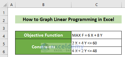
Suppose we have the following objective function:

F = 6X+8Y

And two constraints:
- Constraint 1:

2X+4Y <= 60

- Constraint 2:

4X+2Y <= 48

Now, you can find the optimum point by graphing the linear programming in Excel by using the following steps below.

Required Data to Graph Linear Programming in Excel

Step 1 – Record Objective Function & Constraints Line Points

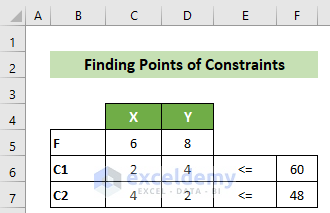
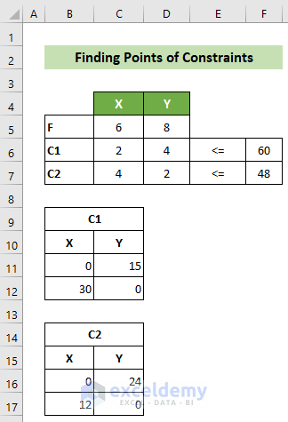
Note down the coefficients and symbols for your objective function and constraints.

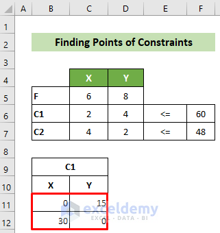
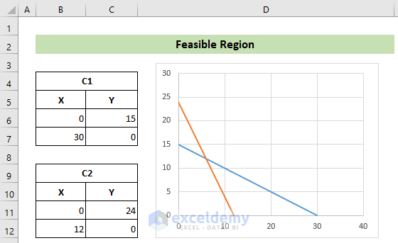
Recording the Functions and Constraints to Graph Linear Programming in Excel

For the first constraint (C1), find two points on the equation. Set X=0 to get Y=15, and set Y=0 to get X=30.

Constraint 1 Line's Points

Similarly, find two points for the second constraint (C2). Setting X=0 gives Y=24, and setting Y=0 gives X=12.

Constraint 2 Line's Points

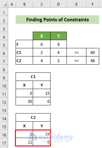
Create a worksheet with your objective function, constraints, and these two points. The worksheet will look like this:

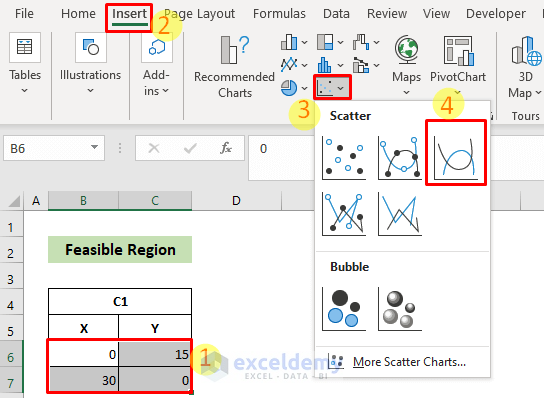
Objective Function with Constraint Points

Step 2 – Determine the Feasible Region

Select cells B6:C8.
Go to the Insert tab, choose Scatter or Bubble Chart, and select Scatter with Smooth Lines.

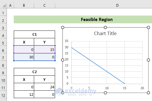
Insert Scatter Plot to Graph Linear Programming in Excel

The resulting scatter plot will not be in the desired format.

Inserted Plot

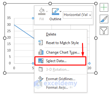
Right-click on the chart, choose Select Data.

Accessing the Select Data Source Window

Choose the series1 option.

Accessing the Edit Series Window

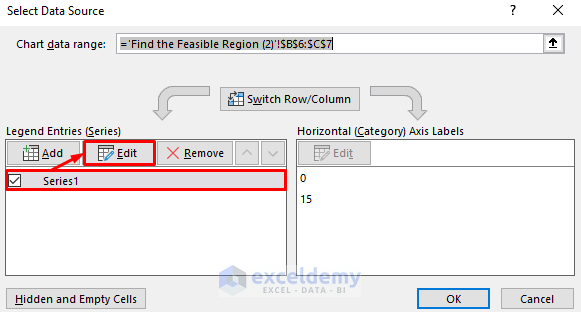
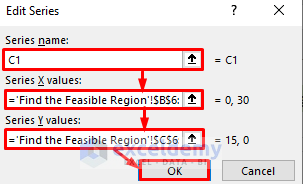
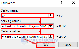
Edit the series by naming it “C1” and specifying the X and Y values from B6:B7 and C6:C7, respectively.
Click on the OK button.

Edit Data Series for the Constraint Scatter to Graph Linear Programming in Excel

In the Select Data Source window, click on the Add button.

Adding Another Data Series

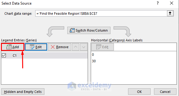
Add another series named “C2” with X values from B11:B12 and Y values from C11:C12.

Edit the Data Series for Added Constraint Plot

Click on the OK button.

Finalize the Plot to Graph Linear Programming in Excel

Confirm your selections and create the scatter graph.

Constraint Graphs

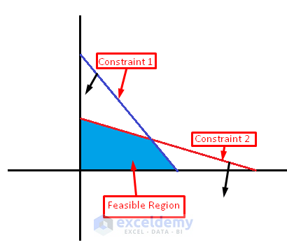
Since both constraints are less than or equal inequalities, the feasible area will be bounded by the lines and directed toward the origin.

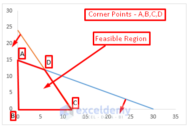
Find the Feasible Region to Graph Linear Programming in Excel

The resulting graph should resemble the figure provided, with ABCD representing the feasible region, and A, B, C, and D as the corner points.

Step 3 – Determine the Optimum Solution

After identifying the feasible region, the next step is to find feasible solutions.

Locate the X and Y coordinates of the corner points. From the graph and constraint value table, we can easily identify points A (0,15), B (0,0), and C (12,0).

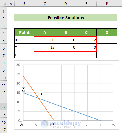
Feasible Solutions from Graph & Axis

To find the coordinates of point D, select cells D5:D6 and enter the following formula involving the MMULT and MINVERSE functions:

=MMULT(MINVERSE('Finding Points of Constraints'!C6:D7), 'Finding Points of Constraints'!F6:F7)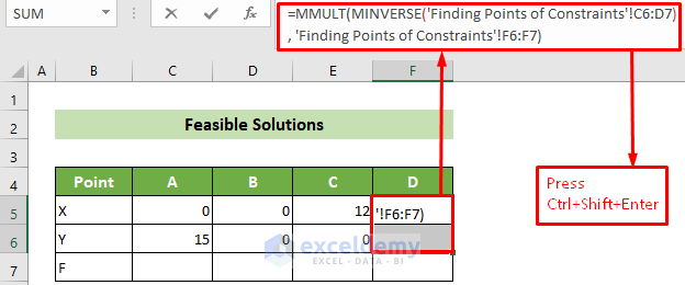

Find the Remaining Feasible Solution through MMULT and MINVERSE Functions

Formula Breakdown

MINVERSE(‘Finding Points of Constraints’!C6:D7)

The MINVERSE function calculates the inverse matrix of the values in the Finding Points of Constraints worksheet (C6:D7)

Result: The result provides the coordinates of point D: (-0.166666667, 0.333333333) and (0.333333333, -0.166666667).

=MMULT(MINVERSE(‘Finding Points of Constraints’!C6:D7), ‘Finding Points of Constraints’!F6:F7)

This returns the matrix product of the previous result’s array and the Finding Points of Constraints worksheet’s F6:F7 array.

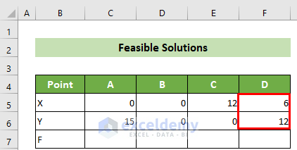
Result: {6,12}

As a result, you will get the coordinates of the intersecting point D of the two constraint lines.

Remaining Feasible Solution to Graph Linear Programming in Excel

With all corner points identified, proceed to find feasible solutions. In cell C7, enter the formula:

=(C5*'Finding Points of Constraints'!$C$5)+('Finding Points of Constraints'!$D$5*C6)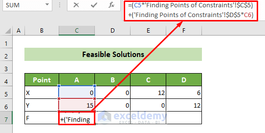

Find Objective Function's Values to Graph Linear Programming in Excel

Formula Breakdown

=(C5*’Finding Points of Constraints’!$C$5)

This will calculate the multiplication of the C5 cell value and the Finding Points of Constraints worksheet’s C5 cell value.

Result: 0

(‘Finding Points of Constraints’!$D$5*C6)

This will multiply the Finding Points of Constraints worksheet’s D5 cell value with the C6 cell value of the current worksheet.

Result: 120

=(C5*’Finding Points of Constraints’!$C$5)+(‘Finding Points of Constraints’!$D$5*C6)

This will sum up the previous two results.

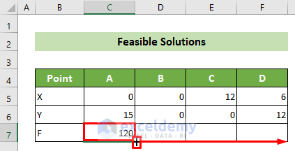
Result: 120

Drag the fill handle in the bottom right corner of the cell to copy the same formula for other points, obtaining all feasible solutions.

Drag Fill Handle to Copy Formula

As a result, you will get all the feasible solutions.

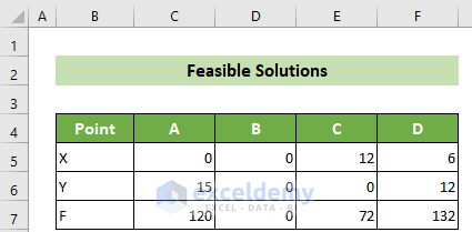
All Feasible Solution of Linear Programming

To solve your linear programming problem, find the maximum value of F. At point D (6,12), the maximum value of F is 132, making it the optimum solution.

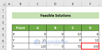
Optimum Solution of Linear Programming

Your linear programming process using the graph concludes with this final result.