How to Calculate Shadow Price Linear Programming in Excel

Get FREE Advanced Excel Exercises with Solutions!

In this article, we will learn how to calculate shadow price linear programming in Excel. The Shadow Price is the change in the value of the objective function per unit increase in the constraint. It is a very important tool for financial calculations. In industry, we need to know these parameters before producing products. We can easily do this task in Excel. So, without any delay, let’s start the discussion.

Table of Contents hide

Download Practice Workbook

Step-by-Step Procedures to Calculate Shadow Price Linear Programming in Excel

STEP 1: Prepare Dataset

STEP 2: Use Solver Feature to Calculate Shadow Price Linear Programming

STEP 3: Get Answer & Sensitivity Report

Practice Section

Conclusion

Download Practice Workbook

To practice by yourself, download the following workbook.

Shadow Price Linear Programming.xlsx

Step-by-Step Procedures to Calculate Shadow Price Linear Programming in Excel

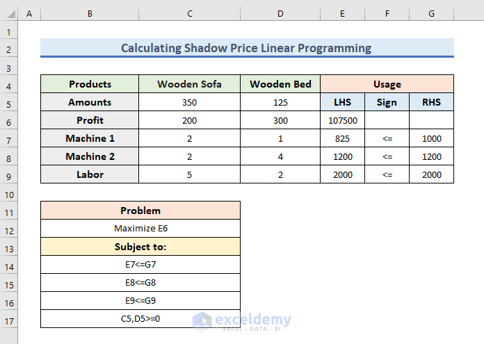
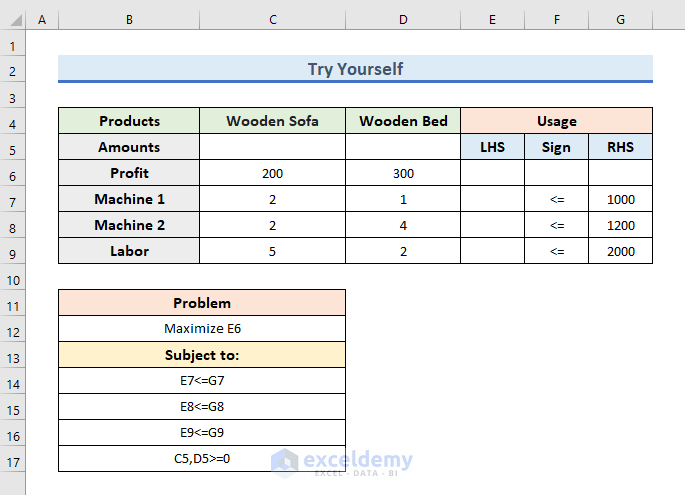
To demonstrate the method, we have taken the following dataset. The dataset contains information on a wood shop where Wooden Sofas and Wooden Beds are made. The shop gets 200 and 300$ benefits per Sofa and Bed respectively. But, there are some constraints. From this dataset, we will find out the maximum profit. After that, we will calculate the shadow price with linear programming.

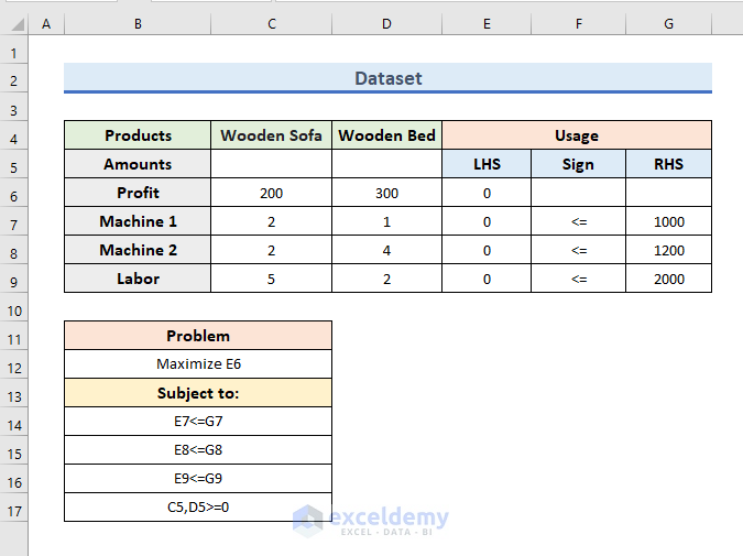
Let’s follow the steps below to learn the method.

STEP 1: Prepare Dataset

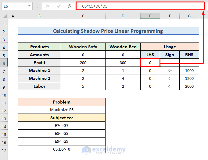
First, we need to prepare our dataset with some modifications to solve the problem. We will link up between cells using the formulas.

Firstly, we have to insert the formula of total profit.
To do so, write down the following formula in the E6 cell:

=(C6*C5)+(D6*D5)

Then, press Enter to get the result.
Now, it is showing 0.
But after solving this, we will get the maximum profit in this cell.

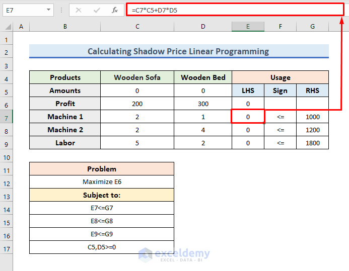
Now, write down the following formula in the E7 cell:

=C7*C5+D7*D5

Then, press Enter to proceed.
From this cell, we will get the LHS (Left Hand Side) of a constraint.

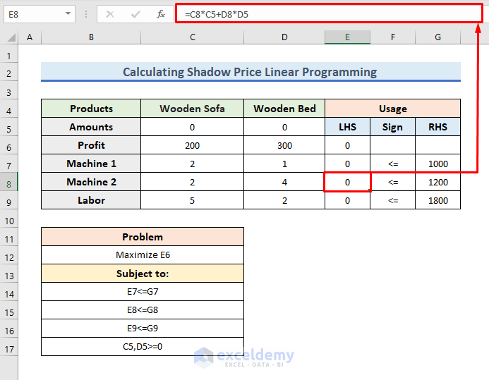
Now, write down the following formula in the E7 cell:

=C8*C5+D8*D5

Then, press Enter to proceed.
From this cell, we will get the LHS (Left Hand Side) of another constraint.

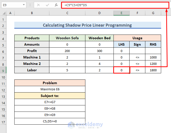
Now, write down the following formula in the E7 cell:

=C9*C5+D9*D5

Then, press Enter to proceed.
From this cell, we will get the LHS (Left Hand Side) of another constraint.

Here, Total Profit which is our objective function comes from the summation of profits of wooden sofas and beds. The total profit of wooden sofas comes from the multiplication of profit per sofa and the number of sofas. Similarly, we can get the profit of the wooden bed by multiplication. After summation of these 2, we can get the total profit. By using the same formula, we have calculated the LHS for these constraints depending on the number of sofas and beds of the constraints.

STEP 2: Use Solver Feature to Calculate Shadow Price Linear Programming

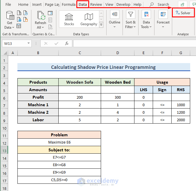
In this step, we will insert the Solver Feature to maximize the objective function. As the by-product of maximization, we will get the shadow price.

Now, we will add a solver in Excel to solve the data.
To do so, click on Data >> Solver to add the solver.

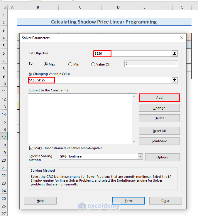
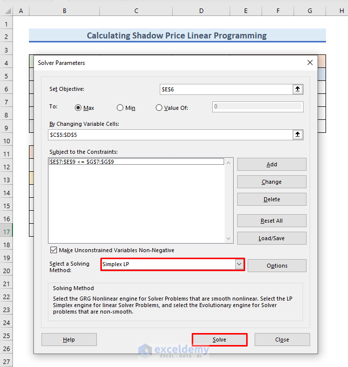
Instantly, you can see a window named Solved Parameters.
Then, we will insert parameters into this window.
So, write $E$6 in the Set Objective field.
Here, the E6 cell indicates the profit of the shop.
After that, in the By Changing Variable Cells field, write down $C$5:$D$5.
Here, these 2 cells are variables.
Then, click on the Add button.

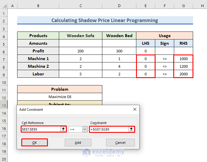
As a result, the Add constraint window will come out.
After that, write according to the following figure.
In the Cell Reference field, write $E$7:$E$9.
And, in the Constraint field, write $G$7:$G$9.
Here, we have declared the constraints.
Then, press OK to proceed.

In this step, we will select the solving method.
So, from the drop-down menu of the Select a solving method, select Simplex LP.
Then, press Solve to solve the problem.

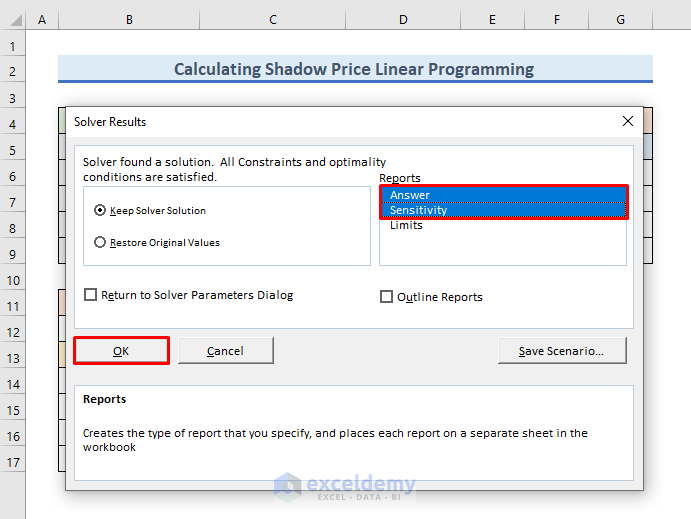
Instantly, you can see a Solver Results window.
Now, in the Reports field, select Answer and Sensitivity and press OK.

STEP 3: Get Answer & Sensitivity Report

We will get 2 Excel Sheets of Answer and Sensitivity reports automatically. From these reports, we will extract our desired information.

Now, you can observe the solution.
Here, you can see the number of Wooden sofas and Wooden Beds for maximum profit.
And, you can watch the total benefit is 107500$.

In the Excel workbook, 2 worksheets have appeared.
First, go to Answer Report 1.
In this report, you can observe the Final Value.
Here, the Final Value means the maximum profit of the shop after maximization.
And, the Cell Value is representing the LHS value of the problem constraint.

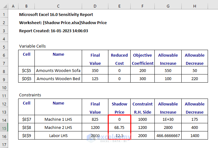
Here, Machine 2 LHS and Labor LHS are binding or limited by the optimization model as Slack is 0. For this reason, if you change these values, then, the optimization parameters will be changed, and maximum optimization will change. So, it will have a shadow price. But, Machine 1 LHS is not binding, so it will not have any shadow price.

After that, go to Sensitivity Report 1.
Then, look for the Shadow Price column.
Here, the Shadow Price is the change in the value of the objective function per unit increase in the constraint’s bound.
As Machine 1 LHS is not binding, it has not any shadow price.

Practice Section

There is a practice Excel Sheet available. You can practise from this sheet.

Conclusion

In this article, we have demonstrated how to calculate shadow price linear programming in Excel. There is a practice workbook at the beginning of the article. Go ahead and give it a try. To read similar articles, check out the ExcelDemy website. Last but not least, please use the comment section below to post any questions or make any suggestions you might have.