How to Do Linear Programming in Excel (2 Suitable Ways)

Linear Programming is one of the most interesting features of applied mathematics. We can solve linear programming through Excel. But Excel has no built-in function or feature to perform this. There are two ways to perform linear programming in Excel, and we will discuss them in detail here.

What Is Linear Programming?

Linear programming is a mathematical term. It is a kind of modeling technique that can achieve the maximum profit or the minimum cost based on the relationships of a linear function. It is also called mathematical optimization.

Introduction to Linear Programming Terms

We will discuss some basic terms of linear programming.

Decision Table: This table consists of some variables to determine the optimum solution to the problem.

Constraints: Those are the conditions imposed on the linear function to get the solutions.

Objective function: This function contains our objective. It is specified as quantitative.

Linearity: The relation between the variable must be linear.

Finiteness: The solution of all the variables must be finite.

Optimal Solution: This is the optimal point of our objective function. From this, we get the values of the variables.

How to Do Linear Programming in Excel: 2 Suitable Ways

There are two ways to do linear programming on Excel. One is by using the graph, and another one is by using an Excel add-in. We will discuss both methods in detail in the next sections.

Suppose, we have the following objective function along with two constraints:

1. Plot Graph to Do Linear Programming

Apply the following steps to solve the linear programming problem by plotting graph.

📌 Steps:

• First, we separate the coefficients of variables.

• Now, we will find out the value of 2 variables considering the value of one variable 0 (Zero). See for the 1st constraint.

When X is 36, Y becomes 0, and when Y is 0, X becomes 18.

Similarly, apply this to the 2nd constraint. Here, X=12 when Y=0 and Y=24 when X=0.

• Similarly, apply this to the 2nd constraint.

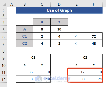
Here, X=12 when Y=0 and Y=24 when X=0.

• Now, select the value from the 1st constraint.
• Click on the Insert tab.
• Choose the desired Scatter Chart from the Chart group.

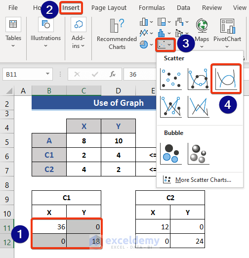
• We will see a graph based on the selection.

• Now, keep the cursor on the chart and press the right button of the mouse.
• Choose Select Data from the Context Menu.

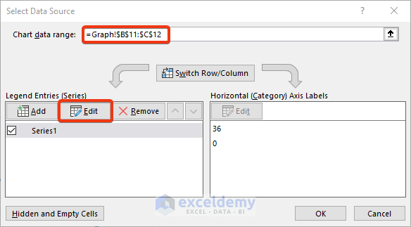
• The Select Data Source window appears.
• Our input data is named Series1.
• We want to change the name.
• Select Series1 and click on the Edit option.

• Put name C1 on the Series name box.
• After that, press OK.

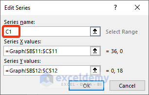
Values of the X and Y are taken from our selection.

• Now, we will add another source as we have another constraint.
• Click on the Add button.

• Now, we will add another source as we have another constraint.
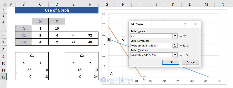
• Click on the Add button.
• The Edit series window appears.
• Put a name, and range for the values of X and Y variables.
• Again, press OK.

• Again, press OK on the next window.

• Look at the graph now.

We have named the edge points.

• Based on the edge points, we form a new dataset table.

We will now find out the position of the intersecting point using a formula. That is point C.

• Put the following formula on Cell E15.

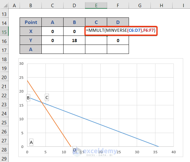
• Press the Enter We get the value of both X and Y coordinates.

• Now, we will find out the optimal value using the formula below.

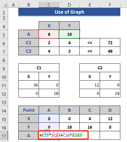
• Press Enter and drag the Fill Handle to the right side.

We get different values of function A for different values of the variables.

At point C, we get the maximum value of A is 192, where X=4 and Y=16.

Read More: How to Graph Linear Programming in Excel (with Detailed Steps)

2. Linear Programming with Excel Add-In

In this section, we will use an Add-in named Solver for this linear system.

📌 Steps:

• First, we separate the coefficients in the following table.

• Now, go to Cell E6 and put the following formula.

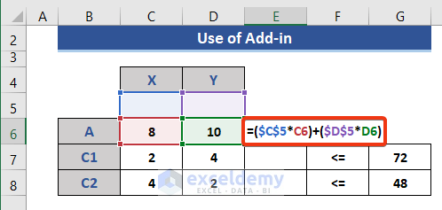
This formula will determine the result of function A.

• Look at the dataset.

As C5 and D5 are blank, the result is 0 (zero). We will expand the formula on Range E7:E8.

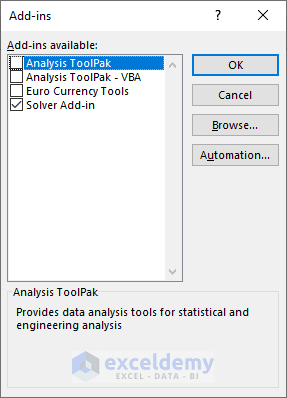
• Now, go to File >> Options >> Add-ins.
• Select the Solver Add-in from the list.
• Then, press Go.
• Check Solver Add-in and then press OK.

• Now, click on Cell E6.
• Click on the Data tab.
• Then, click on the Solver option.

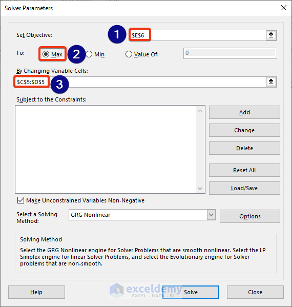
• The Solver Parameters window appears.
• Input objects are marked on the image below.
• Set Objective is the cell we will apply the Solver.
• We want to get the maximum value, so check the Max option. Other options are also available.
• Then, press the Add button.

• We consider those values are equal to or greater than 0. This indicated the value of X and Y.
• Again, press Add to add other constraints.

• This is for the given constraints value input.
• Finally, press OK.

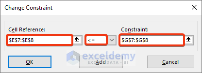
• Both constraints are shown here.
• Now, click on Solve button.

• We get the values of the variable and the function A.

Read More: How to Use Excel Solver for Linear Programming (With Easy Steps)

Download Practice Workbook

Download the following practice workbook to exercise while you are reading this article.

Conclusion

In this article, we described how to do linear programming in Excel. We showed two methods graph and add-in with p[roper explanations. I hope this will satisfy your needs.

Related Articles 

• How to Find Optimal Solution in Linear Programming Excel
• Calculate Shadow Price Linear Programming in Excel
• Perform Mixed Integer Linear Programming in Excel
• How to Do Linear Programming with Sensitivity Analysis in Excel
• How to Solve Transportation Problem with Linear Programming
• Solve Blending Linear Programming Problem with Excel Solver
• How to Solve Integer Linear Programming in Excel