[Fixed!] Excel Superscript Not Working (6 Ideal Solutions)

Sometimes you may set a character as superscript in Excel, maybe want them to appear slightly above the normal line of text. But when you see them in your Excel worksheet, they are in the same line as the text or numbers. There can be various reasons for any superscript not working in Excel.

In this Excel tutorial, we will discuss the reasons for superscripts not working in Excel and provide ideal solutions for them.

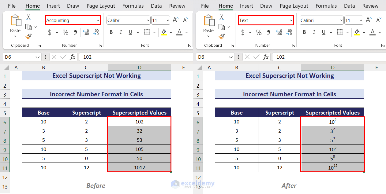
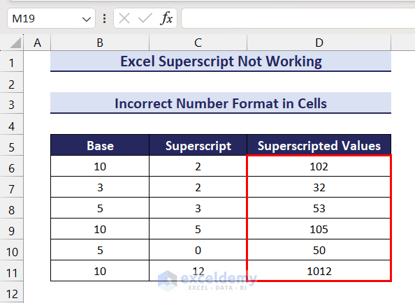
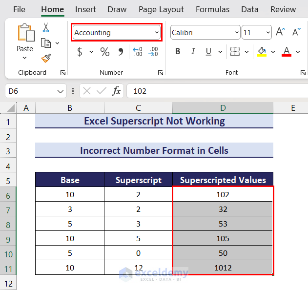
In the following image, we have a dataset where no superscript is not working due to incorrect number formats in Excel. We will demonstrate how to fix this issue and get superscripts in Excel.

Click the image for a detailed view.

When you manually set a character as superscript as General, Text, or Currency. If any other number format is used, the characters will not be displayed as superscripts. Sometimes you may try to insert superscripts using their Unicode values and CHAR function. In such cases, you will get #VALUE! error for superscript characters other than ¹, ² & ³.

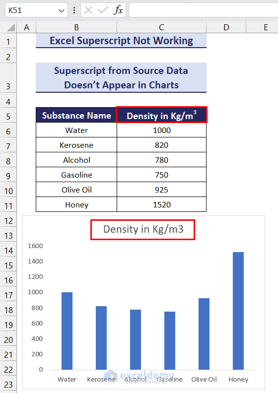
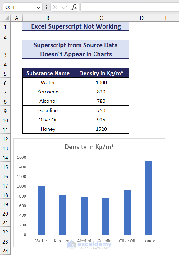
If superscripts are set using the Format Cells dialog box in source data, they will not appear in Excel charts.

Note: We used Microsoft 365 to prepare this article. However, you can find the features and functions used in this tutorial in Excel 2021, Excel 2019, Excel 2016, and Excel 2013 versions as well.

Reason 1: Superscript Not Working Due to Incorrect Number Format in Cells

In the following simple dataset, we have set some characters as superscripts from the Font tab of the Format Cells dialog box. However, the superscripts are still displayed as normal characters.

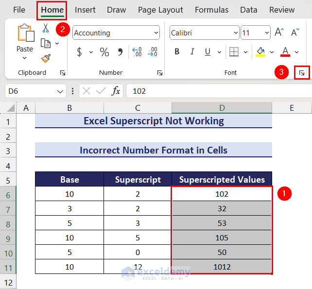
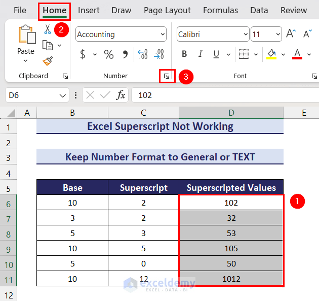
Let’s check whether the Superscript format is still enabled. Select the range D6:D11 => go to the Home tab => you will notice the Format Cells dialog box launcher icon under the Font group of commands.

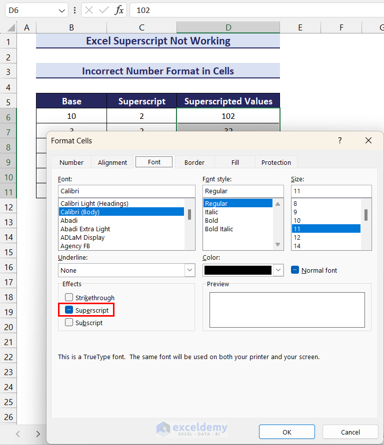
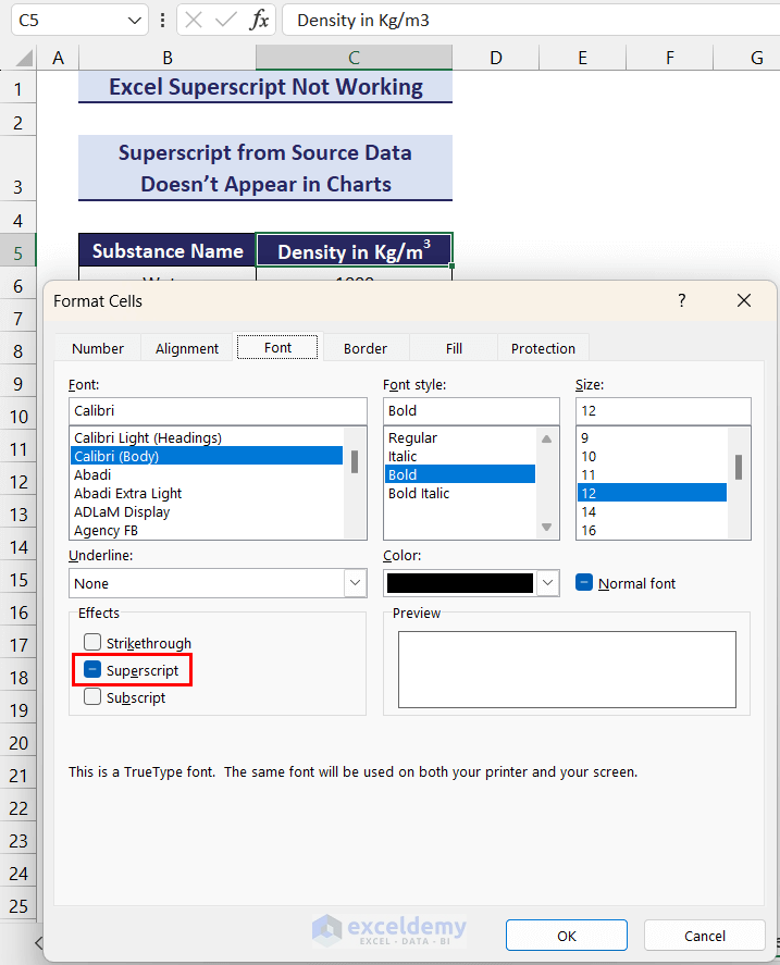
After clicking the dialog box launcher icon, you will get the Font tab of the Format Cells dialog box. As you can see, the Superscript effect is still enabled.

Click the image for a detailed view.

The reason for the Superscript effect not working here is incorrect number formatting in Excel. If you check the Number Format of the range D6:D11, you will notice they are formatted as Accounting.

Read More: How to Add Superscript in Excel

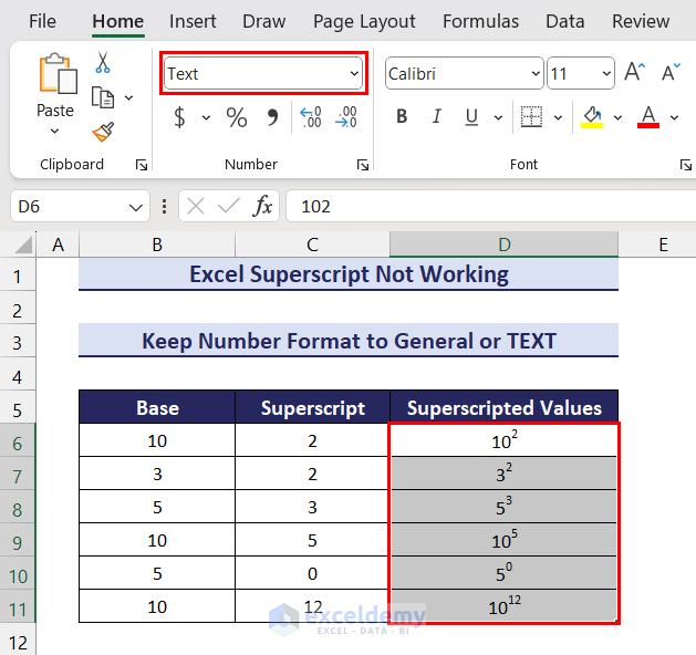
Solution 1: Change the Number Format to General, Text, or Currency

For the Superscript effect to work, you have to set the Number Format to General, Text, or Currency. Other number formats will always or occasionally show inaccurate results.

Apply the steps below to set the proper number format and show superscripts.

Step 1: Select the range D5:D11 => go to the Home tab => you will see the Format Cells dialog box launcher icon under the Number group.

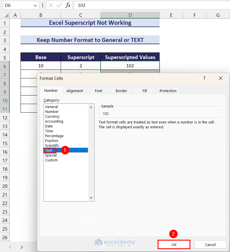
Step 2: After clicking the dialog box launcher icon, you will get the Number tab of the Format Cells dialog box. Set the Category to General, Text, or Currency.

Here, I will set the Category to Text.

You can click the image for a detailed view

Step 3: Click the OK button. As the Number Format is now set to Text, the superscripts will work properly as well.

Read More: How to Write 1^st 2^nd 3^rd in Excel

Solution 2: Apply VBA Code to Generate Superscript

We can apply a VBA code to change the number format of a range of cells and apply the Superscript effect as well. Apply the steps below to generate superscripts with a VBA code.

Step 1: Go to the Developer tab. You will see the Visual Basic option under the Code group of commands.

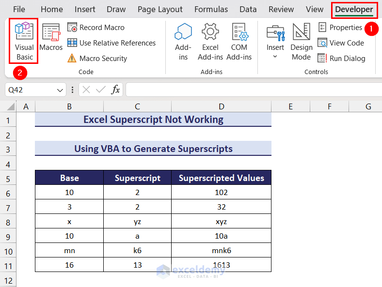
Step 2: After clicking the Visual Basic command, the Visual Basic Editor window will open. If you click the Insert menu, you will find the Module option.

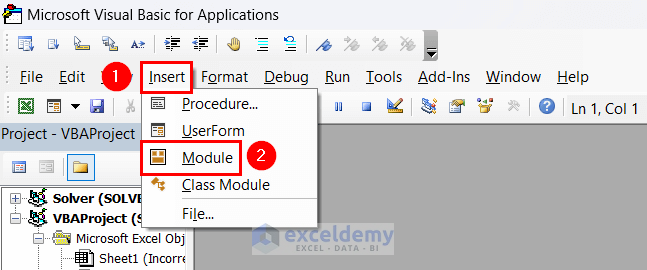
Note: If the Developer tab is not available in your Excel ribbon, then you can use the keyboard shortcut Alt + F11 to open the Visual Basic Editor window.

Step 3: After selecting the Module option, Module1 will appear. Insert the following code in the module and click the Save button.

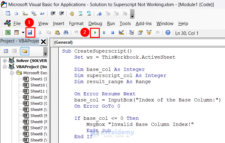
Sub CreateSuperscript()
    Set ws = ThisWorkbook.ActiveSheet
    
    Dim base_col As Integer
    Dim superscript_col As Integer
    Dim result_range As Range
    
    On Error Resume Next
    base_col = InputBox("Index of the Base Column:")
    On Error GoTo 0
    
    If base_col <= 0 Then
        MsgBox "Invalid Base Column Index!"
        Exit Sub
    End If
    
    On Error Resume Next
    superscript_col = InputBox("Index of the Superscript Column:")
    On Error GoTo 0
    
    If superscript_col <= 0 Then
        MsgBox "Invalid Superscript Column Index"
        Exit Sub
    End If
    
    On Error Resume Next
    Set result_range = Application.InputBox("Select the output range:", "Select Range", Type:=8)
    On Error GoTo 0
    
    If Not result_range Is Nothing = False Or result_range.Columns.Count > 1 Then
        MsgBox "Invalid Output Range!"
        Exit Sub
    End If
    
    
    Dim i As Integer
    Dim base As String
    Dim super_script As String
    Dim adrs As String
    
    For Each cell In result_range
        base = ws.Cells(cell.Row, base_col).Text
        super_script = ws.Cells(cell.Row, superscript_col).Text
        cell.NumberFormat = "@"
        cell.Value = base & super_script
        cell.Characters(Start:=Len(base) + 1, Length:=Len(super_script)).Font.Superscript = True
    Next cell
    
End Sub 
			

Step 4: If you click the Run button, you will get an Input Box like the following. Enter the index of the Base column here.

Since the Base values are in Column B, I have entered 2 in the Input Box.

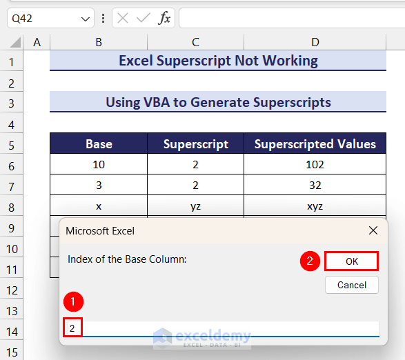
Step 5: After clicking the OK button, you will get another Input Box. Enter the index of the Superscript column here.

Since the Superscript values are in Column C, I have entered 3 in the Input Box.

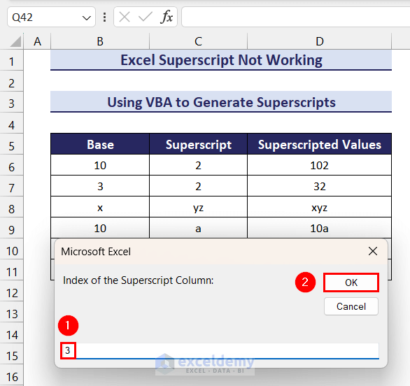
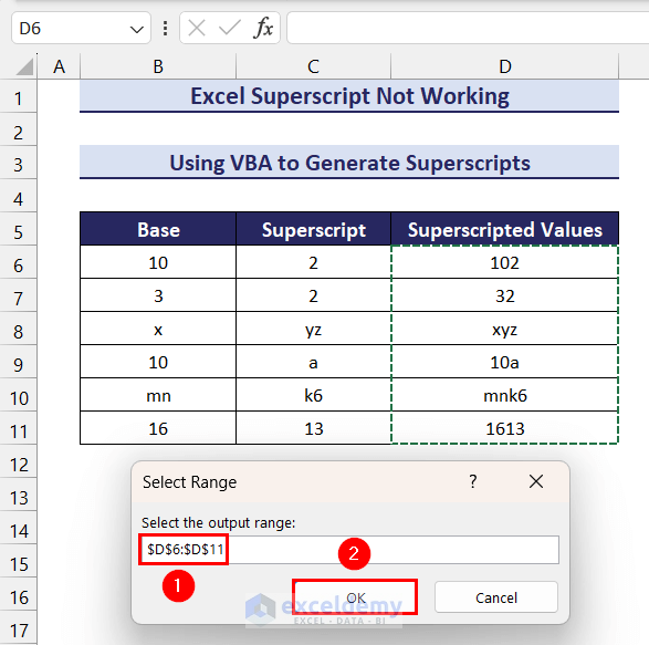
Step 6: After clicking the OK button, you will get one final Input Box for selecting the output range. Select the range D6:D11 here.

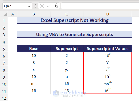
Step 7: After clicking the OK button, return to the worksheet. You will see the output cells have required superscripts now.

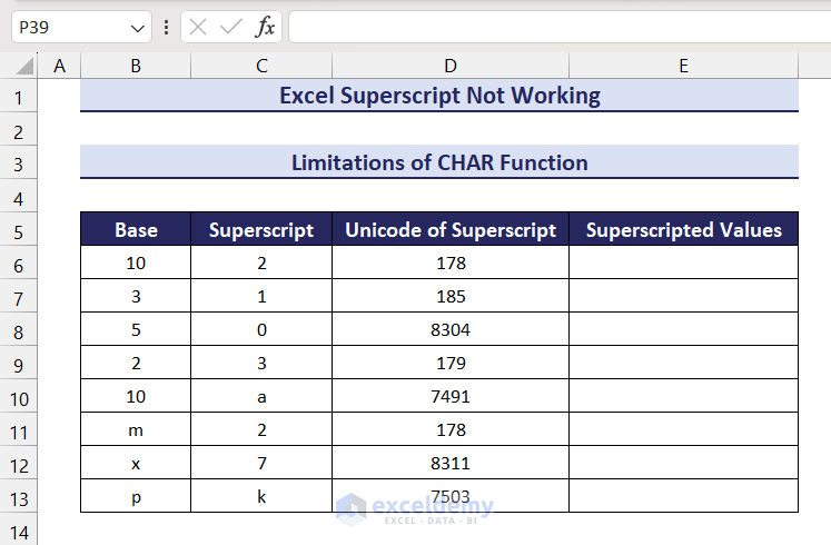
Reason 2: CHAR Function Can Not Generate Superscripts for All Characters

Sometimes you may want to insert superscripts by using the CHAR function. But the CHAR function in Excel takes ASCII codes as its argument, so its arguments are limited between 1 to 255 only. As a result, the CHAR function can return ¹, ² & ³ superscript characters only and shows #VALUE! error for other characters.

For example, consider the following dataset where we have a list of bases, superscripts, and Unicodes for the superscripts.

We can use the following formula in cell E6 to apply superscripts here.

After pressing the Enter key and dragging down the Fill Handle icon, you will get the following output.

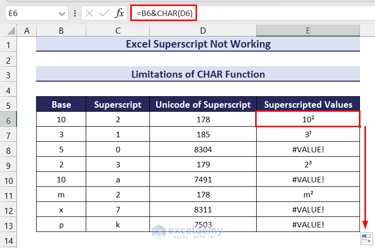
As you can see, we have ¹, ² & ³ superscripts properly, but #VALUE! Error for other characters. We can resolve this problem by using the UNICHAR function or a VBA code instead.

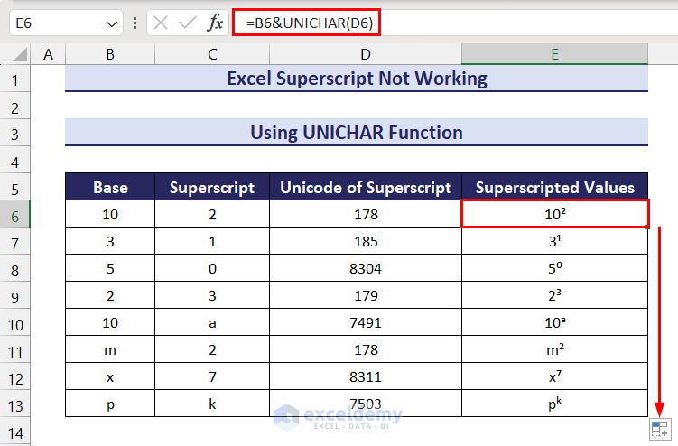
Solution 1: Use UNICHAR Function Instead

Since the UNICHAR function takes Unicode values as its argument, it can return a wide range of superscripts.

To apply superscripts with the UNICHAR function, insert the following formula in cell E6.

Press the Enter key and drag down the Fill Handle icon. This time you will get superscripts for all required characters.

Solution 2: Use Multiple UNICHAR Functions

Although we can generate a wide range of superscripts using Unicodes in the UNICHAR function, there aren’t any Unicodes available for multi-character superscripts. If your superscript contains more than one character or number, you can use multiple UNICHAR functions.

For example, consider the following dataset where the superscript is 25.

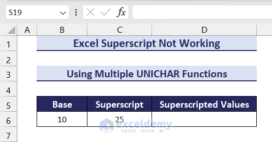
As there is no Unicode for ²⁵, you have to apply two UNICHAR functions with Unicode of ² and ⁵ respectively.

Insert the following formula in cell D6 and press the Enter key to get the required superscript.

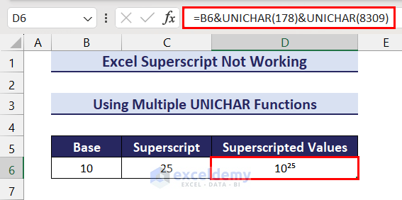
Here, 178 and 8309 are Unicode of ² and ⁵ respectively.

Solution 3: Combine REPT and UNICHAR Functions

If the required superscript has one character multiple times in sequence, you can combine the REPT and UNICHAR functions. For example, consider the following dataset where the superscript is 777. We can use the REPT function to repeat the ⁷ character 3 times.

Type in the following formula in cell D6 and press the Enter key to get the required superscript.

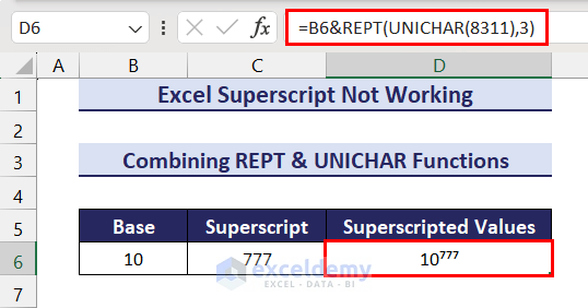
Here, 8311 represents the Unicode of ⁷ character.

The following image contains a list of the Unicodes of the frequently used superscript characters. You can find this list in the practice workbook as well.

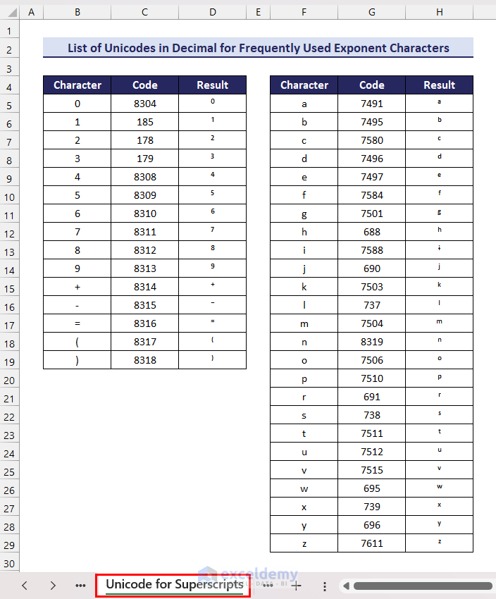
Click the image for a detailed view.

Solution 4: Use VBA to Generate Superscripts

Using the UNICHAR function requires you to know the Unicode of each superscript character. If the superscript contains multiple characters, you have to insert multiple UNICHAR functions. To get rid of these issues, we create a custom VBA function that generates superscripts for frequently used superscript characters. Follow the steps below to learn more about this.

Step 1: Apply the first two steps of Reason 1 Solution 2 section to insert a module. Then, insert the following code in the module.

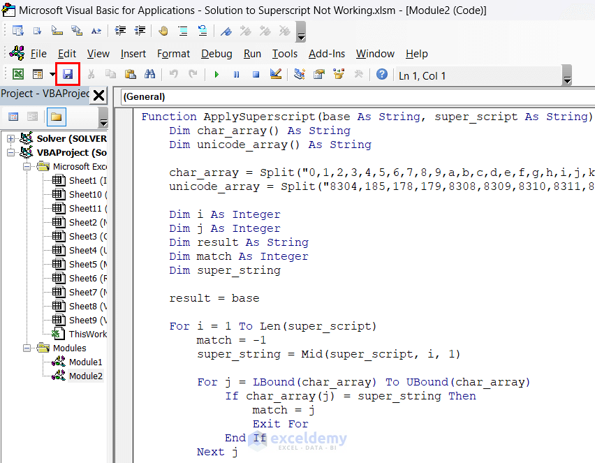
You can click the image for a detailed view

Function ApplySuperscript(base As String, super_script As String) As String
    Dim char_array() As String
    Dim unicode_array() As String
    
    char_array = Split("0,1,2,3,4,5,6,7,8,9,a,b,c,d,e,f,g,h,i,j,k,l,m,n,o,p,r,s,t,u,v,w,x,y,z", ",")
    unicode_array = Split("8304,185,178,179,8308,8309,8310,8311,8312,8313,7491,7495,7580,7496,7497,7584,7501,688,7588,690,7503,737,7504,8319,7506,7510,691,738,7511,7512,7515,695,739,696,7611", ",")
    
    Dim i As Integer
    Dim j As Integer
    Dim result As String
    Dim match As Integer
    Dim super_string
    
    result = base
    
    For i = 1 To Len(super_script)
        match = -1
        super_string = Mid(super_script, i, 1)
        
        For j = LBound(char_array) To UBound(char_array)
            If char_array(j) = super_string Then
                match = j
                Exit For
            End If
        Next j
        
        If match = -1 Then
            result = "Superscript not available"
            Exit For
        End If
        
        result = result & ChrW(unicode_array(match))
    Next i
    
    ApplySuperscript = result
    
End Function 
			

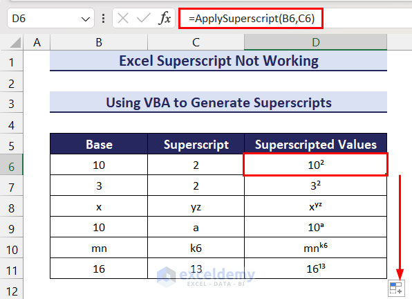
Step 2: Return to the worksheet and apply the following formula in cell D6.

Here, ApplySuperscript is the custom VBA function. The first argument refers to the base and the second argument refers to the superscript.

Step 3: Press the Enter key and use the Fill Handle tool.

What to Do If Superscript Is Not Working in Excel Charts?

Sometimes you may try to load superscripts from source data in chart titles, axis titles, legends, or labels, but get normal characters instead. For example, consider the following dataset where the superscript from the dataset doesn’t appear in the chart.

In the dataset, we had “Density in Kg/m³”, but in the chart title, it shows “Density in Kg/m3”.

This usually happens if the superscript in the dataset is inserted by enabling the Superscript effect from the Font tab of the Format Cells dialog box.

Click the image for a detailed view.

You can insert superscripts from the Symbol feature to get rid of this issue.

Solution: Insert Superscripts from Symbol Feature to Bring Superscript from Source Data to Chart

In the Symbols feature, you can find the superscripts under Latin-1 Supplement, Superscripts and Subscripts, Cyclic Extended-B, Modifier Tone Letters, etc. Subsets. Apply the steps below to add superscript 3 (³) value from the Symbol feature.

Step 1: Select cell C5 => go to the Insert tab => click the Symbols dropdown. You will find the Symbol option.

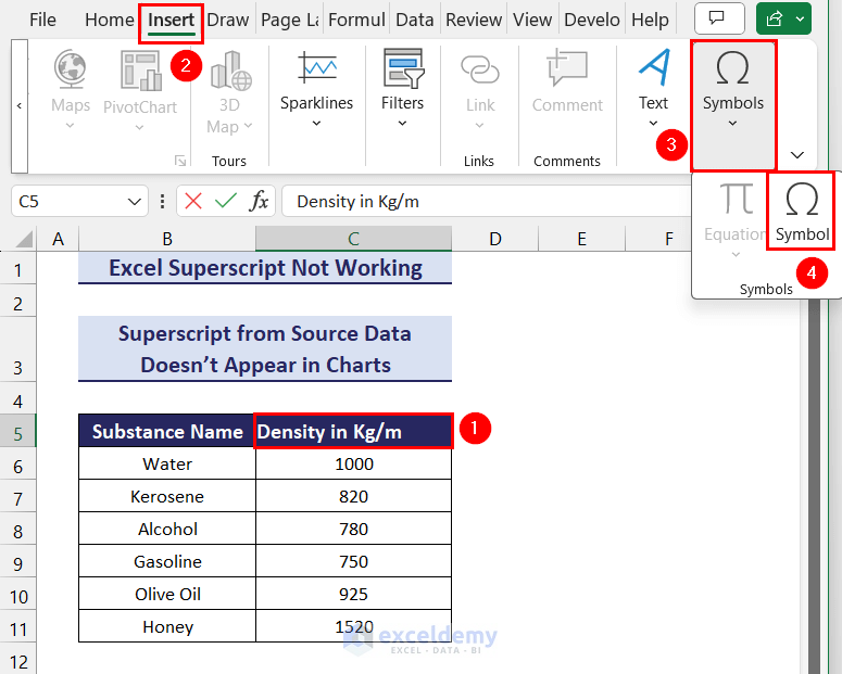
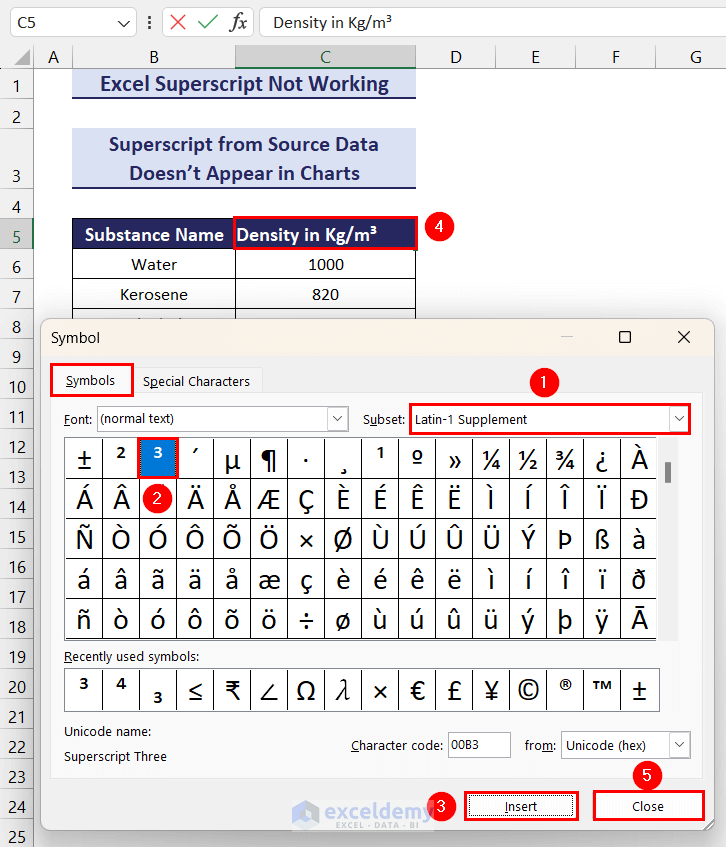
Step 2: If you click the Symbol option, you will get the Symbols tab of the Symbol dialog box. For superscript 3 (³) character, set the Subset to Latin-1 Supplement => select the ³ symbol => click the Insert button. You will get the ³ symbol in cell C5.

You can click the image for a detailed view

Step 3: Finally, click the Close button and the required superscript from the source data will appear in the Chart as well.

Read More: [Solved:] Excel Subscript Not Working

Download Practice Workbook

Back to Learn Excel > Formatting Text > Subscript and Superscript

This concludes our tutorial on superscript not working in Excel. We discussed how incorrect number formatting in cells and limitations of the CHAR function can lead to any superscript not working in Excel. It also showed ideal solutions to get rid of these issues by applying proper number formats, using the UNICHAR function, or applying VBA codes.

We also discussed why superscripts from source data do not appear in Excel charts and how to fix this. We hope that the solutions we provided were helpful to you. Let us know your feedback in the comment section.

Related Articles

• How to Write Subscript in Excel
• How to Write CO₂ in Excel
  

<< Go Back to Subscript and Superscript | Text Formatting | Learn Excel