How to Use REPT Function in Excel (8 Suitable Examples)

In Microsoft Excel, the REPT function is generally used to repeat a text or a character a defined number of times in a cell. In this article, you’ll get to learn how you can use this REPT function effectively in Excel with appropriate illustrations.

The above screenshot is an overview of the article, representing a few applications of the REPT function in Excel. You’ll learn more about the methods along with the other functions to use the REPT function precisely in the following sections of this article.

Introduction to the REPT Function

• Function Objective:

The REPT function is used to repeat text a given number of times. 

• Syntax:

=REPT(text, number_times)

• Arguments Explanation:

• Return Parameter:

Repeated number of the selected text or character in a cell.

How to Use REPT Function in Excel: 8 Suitable Approaches

1. Basic Use of REPT Function in Excel

In Column B, there are some characters or texts and in Column C, the number of times those characters or texts have to be repeated is lying. We’ll find the outputs in Column D.

With proper arguments input, the related formula in Cell D5 will be:

After pressing Enter, you’ll find the asterisk (*) defined number of times.

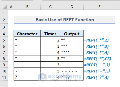
Or if you want to use cell references for the arguments, then you have to type:

2. Replacing Characters in a Text with REPT Function

If you want to replace all the characters in a text with a repeated number of another particular character or text, then the following example in the screenshot should meet the requirement.

The related formula in the output Cell C5 will be:

Press Enter and you’ll be shown the result at once.

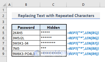
In this formula, the LEN function defines the number of times of the output character which is based on the length of the characters of all texts in Column B.

3. Creating Ratings Based on Review Counts with REPT Function

By applying the REPT function, you can easily create ratings of a product based on the review counts. In the picture below, Column F shows the output ratings based on the ratio between positive and total review counts on a scale of 10.

The required formula to find the rating for the first product in Cell F5 should be:

Press Enter and the formula will return 8 star characters as the rating for the first product.

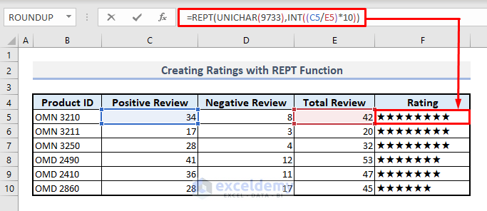
In this formula, the text character in the first argument has been defined by the UNICHAR function with a code- 9733 which is assigned to the symbol of a  black star. In the second argument, the rating in a numerical value has been inputted.

4. Generating Tally Chart with REPT Function in Excel

With the combination of REPT and other suitable functions, you can create a tally chart too for several data counts. In Column D, the tally counts represent the number of sales for each salesman.

For the first one, the required formula to generate the tally count should be:

After pressing Enter and changing the font into Century Gothic, you’ll be displayed the desired output.

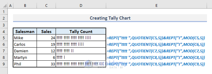
In this formula, “tttt” text has been used to show a single and complete tally sign that denotes the count of 5 instances. With the uses of QUOTIENT and MOD functions, the total counts of complete and incomplete tally signs have been defined.

5. Extracting Last Text Value from a Range of Cells with REPT Function

If you need to extract the last text value from a range of cells in a column, the combination of the VLOOKUP and the REPT functions should serve the purpose. In Column B, there are several random product IDs and we’ll pull out the last text value from this column.

So, our required formula in the output Cell D9 will be:

Press Enter and the resultant output will return right away.

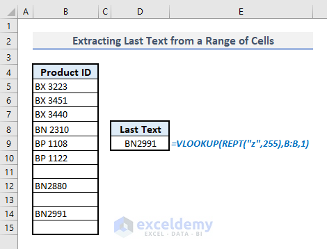
Here, inside the VLOOKUP function, the REPT function creates a string of 255 characters with the last character of English alphabets. When the VLOOKUP function looks for this criterion in the column, it will return the last text data from the column with the approximate match.

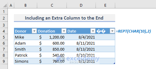
6. Including an Extra Column to a Table with REPT Function

In the picture below, a random table with some data is present. We want to add an extra column to the end of the table.

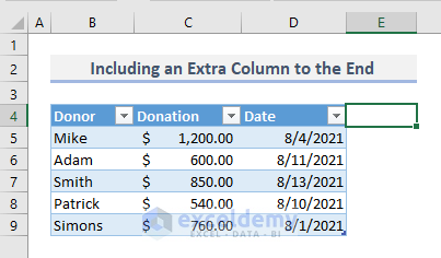
The related formula with the REPT function in Cell E4 will be:

After pressing Enter, you’ll find a new column with empty cells at once.

7. Adding Leading Zeros with REPT Function

The REPT function is useful when you have to add leading zeros to a range of numbers to make all the numbers equal in length.

Based on the random integer numbers in Column B, the required formula to keep all digits in five characters for the first one will be:

Press Enter and you’ll be shown three zeros(0) before the selected number 35.

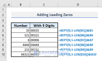
In this formula, “5-LEN(B5)” defines the number of zeros to be added before each number from Column B. With the use of Ampersand(&), the zeros and the selected numbers in Column B have been concatenated.

8. Splitting a Sentence by a Common Delimiter with REPT Function

In Cell B5, a random sentence is lying and we can split all words in the sentence with a particular delimiter- space. The required formula with the help of REPT function in the output Cell B8 will be:

After pressing Enter and auto-filling the bottom three cells with Fill Handle, you’ll find all the split words in the column.

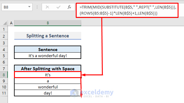
🔎 How Does the Formula Work?

➤ SUBSTITUTE(B$5,” “,REPT(” “,LEN(B$5))): Inside the MID function, this part of the formula replaces all the spaces found in the sentence with the number of more spaces based on the length of the character of the entire text string. This formula thereby returns:

“It’s                     a                     wonderful                     day!”

➤ (ROWS(B5:B$5)-1)*LEN(B$5)+1: The second argument (start_num) of the MID function defines the starting number of each word in the sentence and for four separate words will be 1,2,3 and 4.

➤ LEN(B$5): The third argument (num_chars) of the MID functions has been defined by the length of all characters in Cell B5.

➤ With all three arguments mentioned above and separately, the MID function returns-

“It’s                 “

➤ The TRIM function then removes all unnecessary spaces from the previous output found by the MID function.

➤ While using Fill Handle for the bottom three output cells, the start_num or starting number of each word changes with the change of row numbers for the MID function and thus displays the rest of the words from the sentence in the next three defined cells.

💡 Things to Keep in Mind

🔺 In the second argument (number_times) of the REPT function, the number has to be in integer form otherwise, it’ll be truncated to the integer.

🔺 If the second argument is zero(0), the function will return an empty string.

🔺 REPT function is really useful when you have to create an In-Cell data chart without using Conditional Formatting.

🔺 REPT function can return values up to 32767 characters.

Download Practice Workbook

You can download the Excel workbook that we’ve used to prepare this article.

Concluding Words

I hope all of the suitable methods mentioned above to use the REPT function will now provoke you to apply them in your Excel spreadsheets with more productivity. If you have any questions or feedback, please let me know in the comment section. Or you can check out our other articles related to Excel functions on this website.

<< Go Back to Excel Functions | Learn Excel