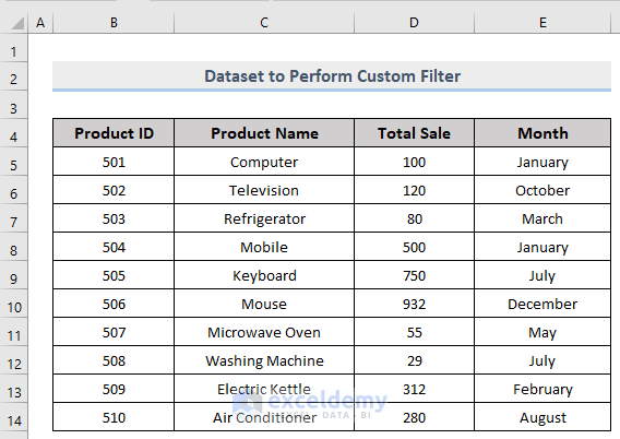
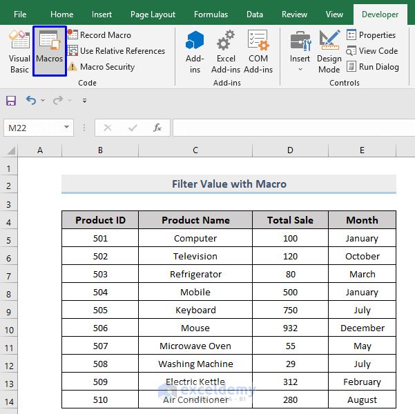
We will use the sample dataset provided below to perform our custom filter.
Method 1 – Filter Value Based on Number in Excel
Steps:
- Select any cell within the range.
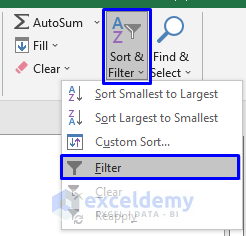
- In the Home tab, select Sort & Filter -> Filter.
- A drop-down arrow will appear next to each column header.
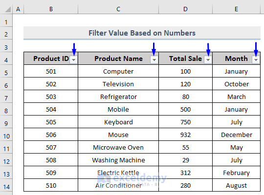
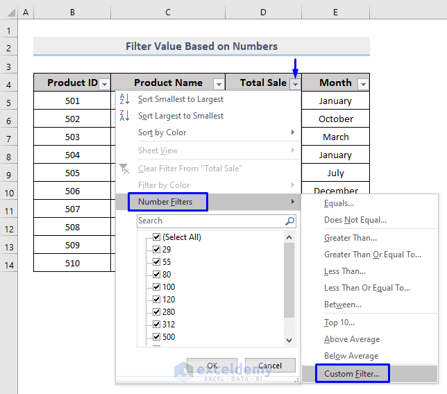
- Click on the arrow next to the column that you want to filter. We wanted to filter based on Total Sales.
- Select Number Filters -> Custom Filter.
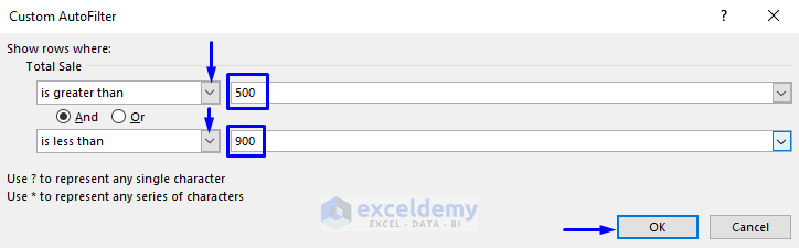
- A Custom AutoFilter pop-up box will appear. Choose the options that you require from the drop-down arrow list. We wanted to extract the Total Sales value between 500 and 900 so we picked is greater than from the first drop-down option and wrote 500 in the label box beside it.
- As we wanted two options to be true so we checked the And option. If you want the result based on only one condition then uncheck And and check Or option.
- From the second drop-down list, we picked is less than and wrote 900 in the label box beside it.
- Press OK.
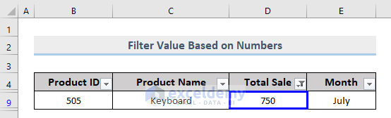
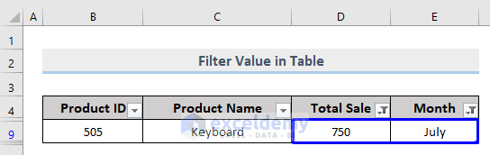
We got the Product details that hold the Total Sale value of 750, which is between 500 and 900.
Method 2 – Filtering Data Based on Specific Text
Similar to the previous section, you can also implement a custom filter to your dataset according to specific text values.
Steps:
- Select any cell within the range.
- In the Home tab, select Sort & Filter -> Filter from the Editing
- A drop-down arrow will appear beside each column header.
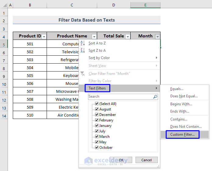
- Click on the arrow beside the column that you want to filter. This time we will filter based on Month.
- SelectText Filters -> Custom Filter.
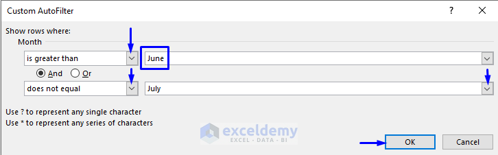
- From the Custom AutoFilter pop-up, choose the options. We wanted to extract the Product details of Months ahead of June except for July, so we picked is greater than and wrote June in the label box.
- We wanted two options to be true, so we checked the And.
- From the second drop-down list, we picked does not equal and selected July to exclude it from the condition. You can also manually enter the month name here.
- Press OK.
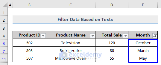
We got the Product details for Months ahead of June except for July.
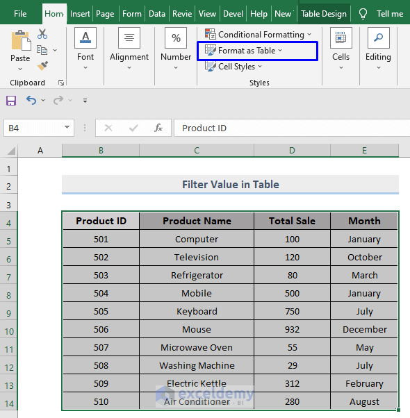
Method 3 – Save Custom Filter in a Table in Excel
Steps:
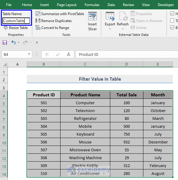
- Give a customized name or leave the name as it is. We have named it CustomTable.
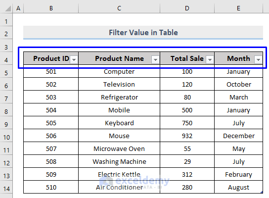
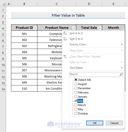
- A drop-down arrow will appear next to each column header.
- Your dataset is now converted as a table with filter options. We wanted to see the Product Details for the month of July, so we unchecked the Select All and checked only July.
- Press OK.
- After extracting only the information for July, we want the Product details that hold the Total Sale value from 500 to 800.
- To filter based on Total Sales, click the drop-down arrow.
- Select Number Filters -> Custom Filter.
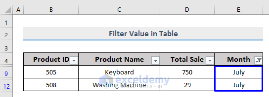
Only the Product details from July will be shown in the table.
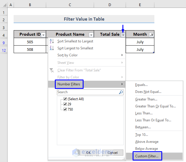
3.1. Execute Custom Filter for Two Columns in a Table
After filtering one column of a table, you can filter another column if you want. We extracted the information for July, and want to get the Product details that hold the Total Sale value from 500 to 800.
- Click on the drop-down arrow next to Total Sales.
- From the drop-down list, select Number Filters -> Custom Filter.
- From the Custom AutoFilter pop-up, we picked is greater than from the first drop-down option and wrote 500 in the label box beside it.
- As we wanted two options to be true, we checked the And
- From the second drop-down list, we picked is less than and wrote 800 in the label box beside it.
- Press OK.
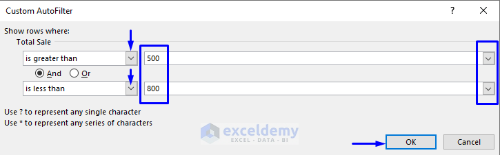
Results show the Product details that were manufactured in July and has a Total Sale of 750 (which is between 500 and 800).
Method 4 – Perform Custom Filter Using Advanced Filter in Excel
Steps:
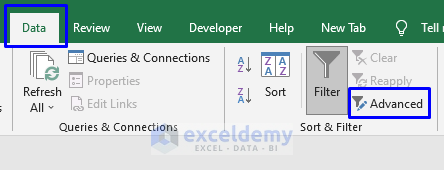
- Select Advanced from the Data tab.
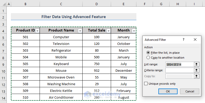
- Advanced Filter has the range of your dataset in the List range.
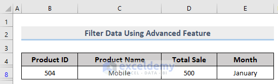
- Go back to the dataset. In another cell, store the data based on which you want to perform the filter. For instance, we wanted to extract data for Mobile, so we stored Mobile in Cell G5 and named the column as Product Name in Cell G4.
- Select the Advanced option, define the Criteria range by dragging the newly defined cells. In our case, we dragged through Cell G4 and G5 as input values in the Criteria range.
- Press OK.
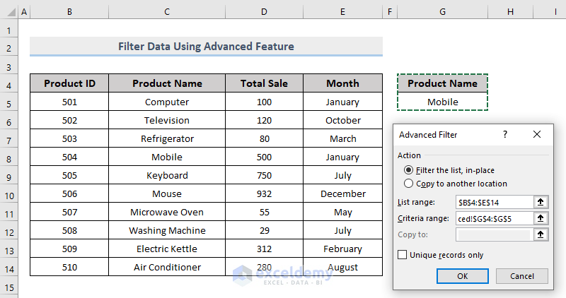
See the details of Mobile in the dataset.
Method 5 – Macro Record to Filter Data in Custom Way in Excel
Steps:
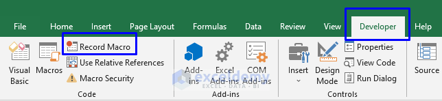
- From the Developer tab, select Record Macro.
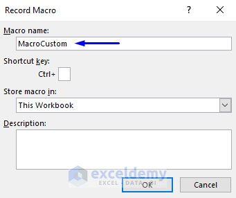
- Name the macro in the Record Macro pop-up box. We named it MacroCustom in the Macro name box.
- Press OK.
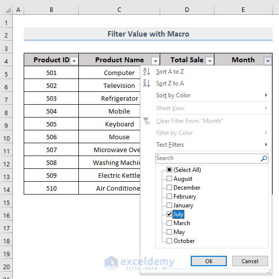
- Now you can perform any type of filter on your dataset. The macro will record your actions and apply the exact same filter to another worksheet. After pressing Record macro, we wanted to extract the Total Sale of July so we unchecked the Select All option and checked July.
- Press OK to show the Product details for July.
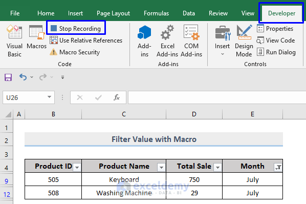
- Select Stop Recording from the Developer tab to record the exact procedure that was followed to filter the data.
- Go to another worksheet that you want to filter. Select Macros from the Developer.
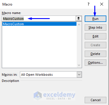
- Select the macro name. For our case, we selected the MacroCustom.
- Press Run.
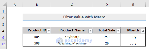
The exact filter process that you followed in the previous worksheet will be applied here.
Download Workbook
<< Go Back to Filter in Excel | Learn Excel
Get FREE Advanced Excel Exercises with Solutions!
