How to Filter Horizontal Data in Excel (3 Methods)

This article explains three methods to filter horizontal data in Excel. Filtering data vertically is easier with the default Filter feature, pivot table, and some other tools. But to filter data horizontally needs to follow some techniques and new functionalities into action.

How to Filter Horizontal Data in Excel: 3 Methods

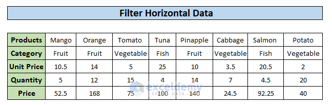
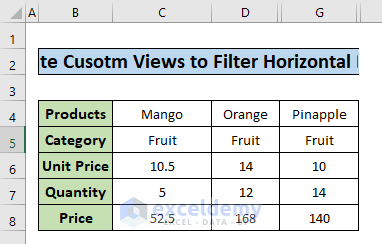
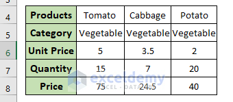
In this article, we’ll use the following dataset. The dataset contains sales data for 8 products that fall into 3 different categories. We will discuss 3 suitable methods to filter this dataset based on categories.

1. Use of the FILTER Function to Filter Horizontal Data in Excel

The FILTER function can perform filter data horizontally easily based on predefined criteria. This function can filter data both vertically and horizontally.

Introduction to the FILTER Function

Syntax:

=FILTER(array, include, [if_empty])
Arguments:

Now, in our example, we are going to filter the dataset based on three different categories i.e., Fruit, Vegetable, and Fish. Let’s follow the steps below.

Steps:

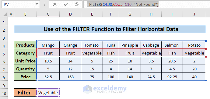
• In cell C10, we put the category name “Vegetable”. We’re going to use this as the criteria to filter the dataset. And we also created an output table to store the filtered data.

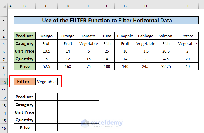
• In the cell, C12 put the following formula.

▶ Formula Breakdown

The FILTER function takes two arguments- data and logic.

• In this formula, cells C4:J8(Blue colored box ) represent data to be filtered. The cells C5:J5 in row C are the categories in the red-colored box from where we set the criteria.
• In the formula, C5:J5=C10 checks the value of cell C10 against each of the cell values of C5:J5. This returns an array, {FALSE, FALSE, TRUE, FALSE, FALSE, TRUE, FALSE, TRUE}. We see that TRUE values are for cells with the category vegetable.

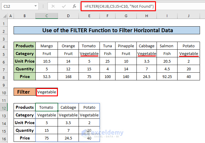
The formula gives a dynamic solution. It means whenever we change cell data the output is going to adjust its value immediately.

• The result shows only the columns with the category Vegetable.

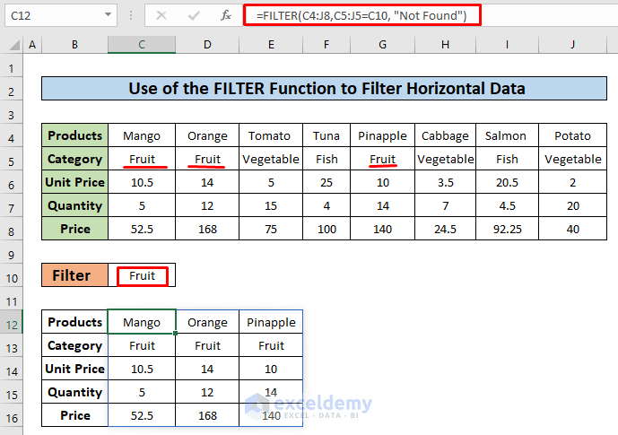
• In this step, we changed the value of cell C10 to Fruit, and the data filtered horizontally for that category accordingly.

2. Transpose and Filter Horizontal Data in Excel

We can transpose our dataset and then use the default filter option that Excel provides to filter horizontal data. Let’s dive into the following example!

Steps:

• At first, select the whole dataset, press Ctrl + C with your keyboard, or right–click the mouse to choose copy from the context menu.

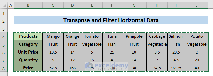
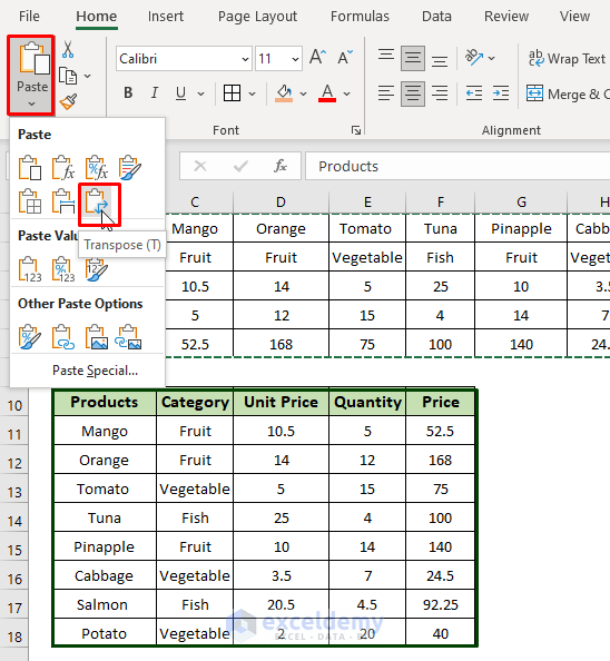
• We need to paste the copied dataset with the Transpose option. Select the cell where you want to paste In this example, we selected cell B10, and then from the Home Tab click on the Paste tab to select the Transpose as paste option.

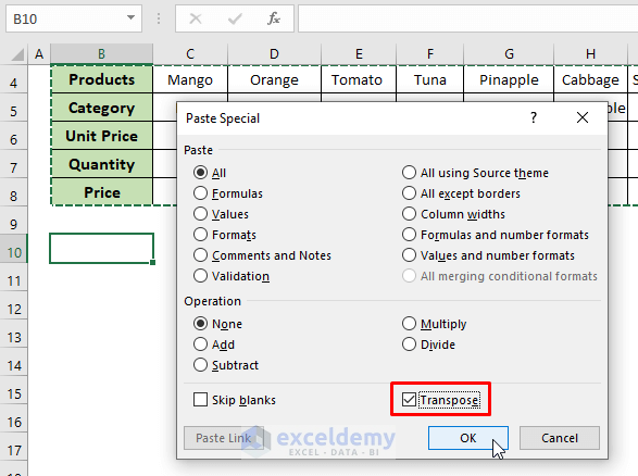
Another Way:

Open up the Paste Special window either from the context menu or from the Home tab. From the Operation options, click the Transpose checkbox and hit OK.

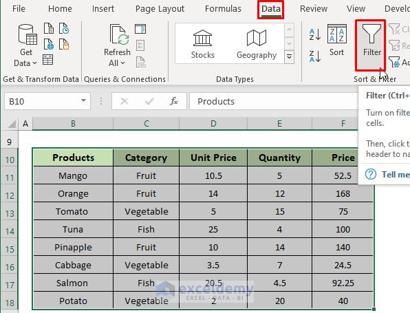
• Now, select the transposed dataset and from the Data Tab click on the Filter option.

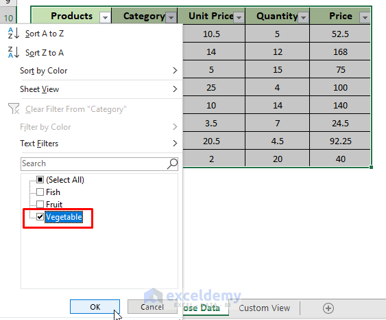
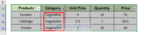
• The above steps enabled filtering options on each of the columns. Click on the Category Filter option and check the Vegetable.

• This is the output we got.

By following the above steps, we can filter the dataset based on any criteria.

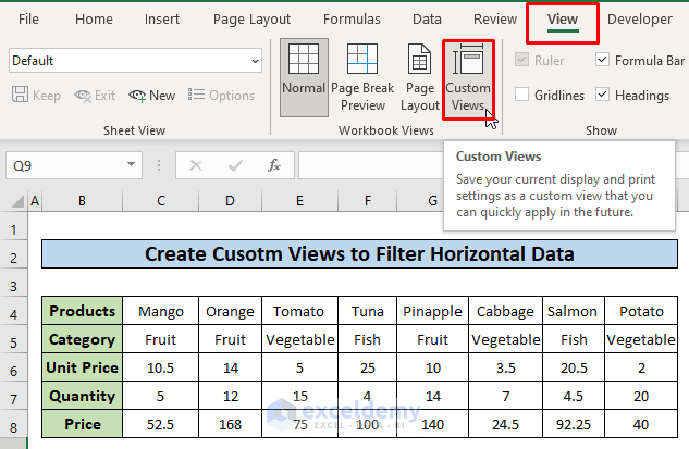
3. Create Custom Views to Filter Data Horizontally in Excel

In this method, we are going to filter horizontal data with the help of  Excel’s Custom Views. We’ll create a number of custom views depending on our criteria. We want to filter data based on the product category. So we need to create 4 custom views in this example. Necessary steps are given below.

Steps:

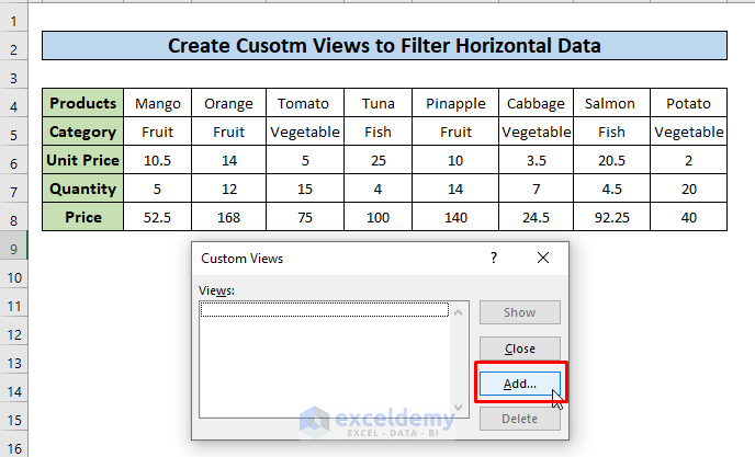
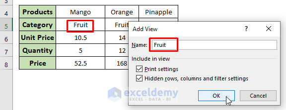
• At first, we are going to create a custom view with the full dataset. Go to the View Tab in the Excel Ribbon and then select the Custom Views option.

• In the Custom Views window click on the Add button.

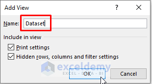
• We put Dataset in the input box as the name of the Custom View and hit

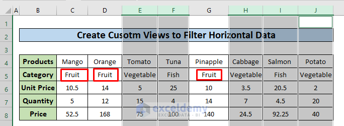
• Now, to create a custom view for the Fruit category, hide all the columns other than the Fruit category. Select the columns E, F, H, I, and J that have data for Vegetable and Fish

• After that, right–click on the top of the column bar and choose Hide from the context menu.

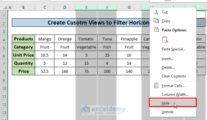
• As a result, all the columns other than the Fruit category are hidden.

• Now, add a custom view named Fruit for the Fruit category.

• Similarly, add another two custom views for the Vegetable and Fish categories named Vegetable and Fish. Finally, we have created 4 custom views.

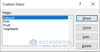
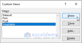
• Now, we can select any of the custom views from the list, and clicking the Show button will show the view for that corresponding product category. For example, we selected the Fish Custom View to show filtered data for the Fish category.

• Here is the filtered dataset for the Vegetable category.

Notes

• The FILTER function is a new function that can only be used in Excel 365. It is not available in the older versions.

Download Practice Workbook

Download this practice workbook to exercise while you are reading this article.

Conclusion

Now, we know how to filter data horizontally in Excel. Hopefully, it would encourage you to use this function more confidently. Any questions or suggestions don’t forget to put them in the comment box below.

<< Go Back to Filter in Excel | Learn Excel