How to Convert Text Filter to Date Filter in Excel (3 Examples)

Among many useful features of Excel in our everyday life, data filtering is one of them. We can insert data filters in Excel through tables, pivot tables, and the filter option from the Data tab. And in our everyday usage, we need to manipulate these filters to our needs. In this article, we will focus on the date filter and how to convert it to one if it is on a text filter in Excel.

How to Convert Text Filter to Date Filter in Excel: 3 Suitable Examples

The method to convert the text filter to a date filter in Excel is simple- you just have to disable the text filter first. Then move on to work with the date filter. If you don’t have the date filter already on, you need to insert one first.

Before we dive deep into the methods, let’s introduce the dataset first.

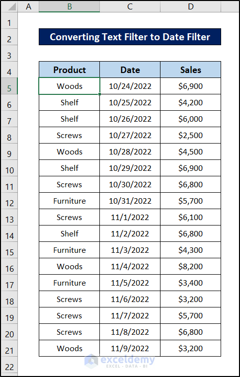
We can have date filters directly on this dataset in two ways- either converting it into a table or a pivot table.

1. Using CheckBoxes in Excel Table

Now let’s suppose we already have one converted. This is the table we are working on first.

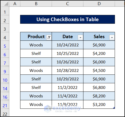
As you can see, the dataset is in a table form already. At the same time, the text filter is on for the “Woods” and “Shelf” values. To convert them into a filter for the date column in this Excel spreadsheet, we first need to disable the text filter (the “product” column). Then we can easily work with the date filter however we want.

Follow these steps to see details.

Steps:

• First, select the filter button beside the column header of the “Product” column.
• Then select Clear Filter from “Product” from the drop-down menu.

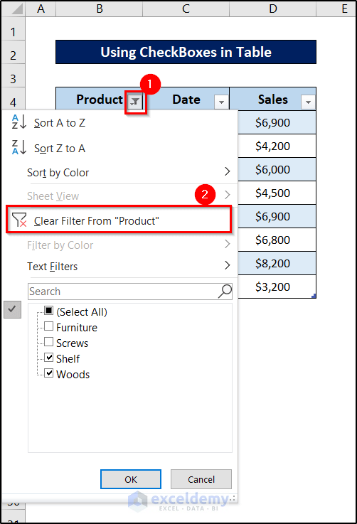
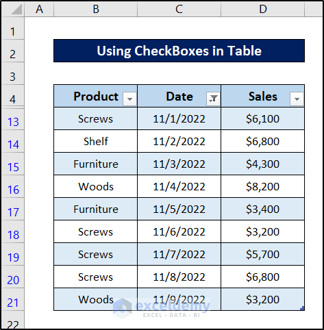
• As a result, this will remove the text filter that already exists in the table.

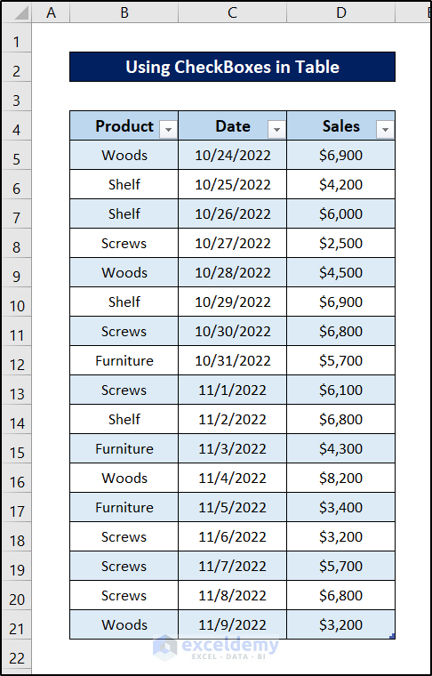
• Next, click on the filter button beside the “Date” Column.
• Then you will see the checkboxes to select/deselect your preferred dates. Now keep the ones you want in the tables checked. And uncheck the ones that you want to hide from the table.

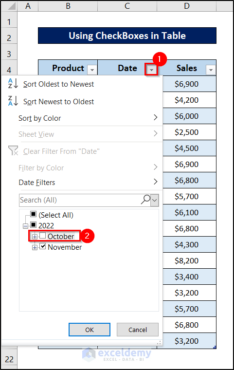
• Once you are done, click on OK.

Thus you can convert an already existing text filter to a date filter table in Excel.

2. Filtering for Specific Date Ranges

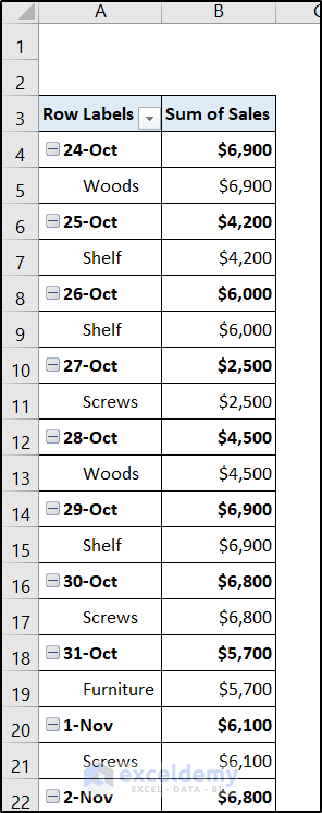
Now let’s take a look at a pivot table made from the same dataset.

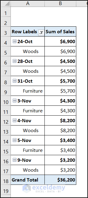
Together with the date values, the text values are already in the pivot table filter. This time, it has the “Woods” and “Furniture” filters on. In a similar fashion to the previous one, we need to convert the text filter to the date filter on the Excel pivot table, but this time, within a specific date range.

Follow these steps to see how you can do that here.

Steps:

• First, select the filter button on the column header of the first column labeled “Row Labels”.
• Then select Clear Filter from Product from the drop-down menu.

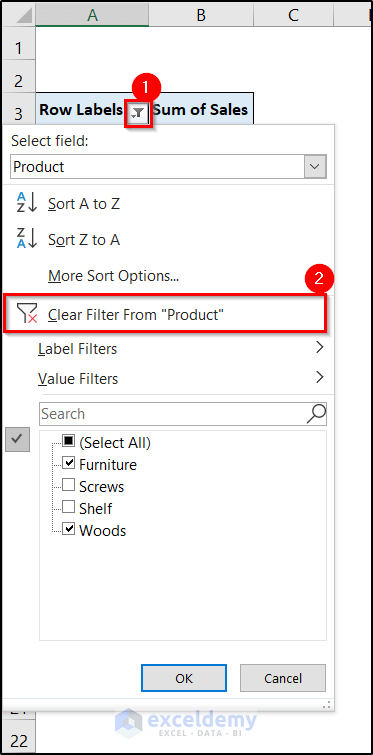
• As a result, Excel will remove the text filters from the pivot table.

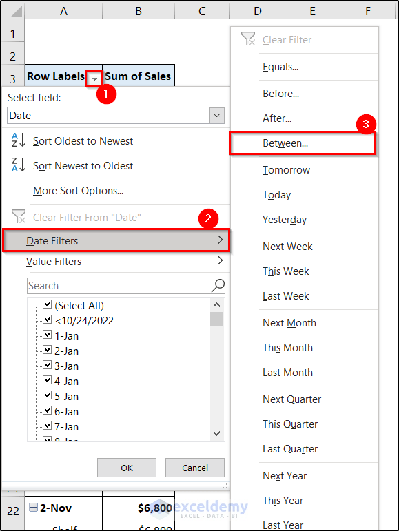
• Now click on the filter button beside the “Row Labels” again.
• But this time, hover your mouse cursor over the Date Filters from the drop-down menu.
• Then select Between from the menu that pops up.

• Next, select is between in the first field of the Date Filter (Date) box that pops up on the spreadsheet.
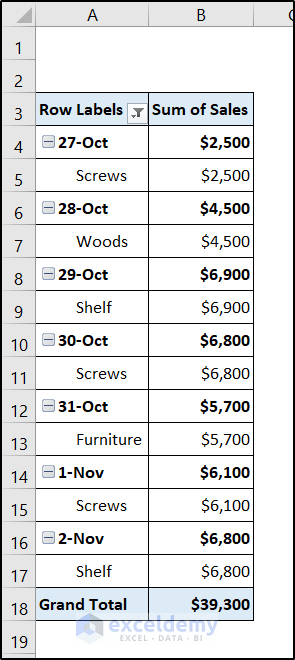
• After that, select the dates between where you want to keep the filtered pivot table in.

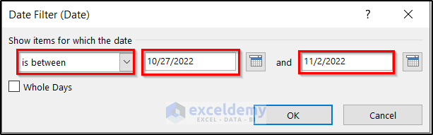
• Finally, click on OK.

And this is how you convert a text filter to a date filter in Excel’s pivot table to keep it in between a range.

3. Applying Date Filter for Dynamic Date Ranges

Next, we will discuss how to use date filters that work with dynamic ranges. As dates are continuously changing, these dynamic filters will help us to reshuffle the data that the pivot table shows depending on the current date. So this is very helpful if we are in constant need of filtering a pivot table if we want them to be in a specific period of time, say on the next month or today’s sales.

Let’s go back to the previous pivot table with the text value filter on. Now we are going to convert the text filter to a dynamic date filter in Excel.

Steps:

• First, click on the filter button beside the “Row Label” on the column header of the first column.
• Then select Clear Filter from Product from the drop-down menu.

• As a result, Excel will clear the text filters from the pivot table.

• Next, click on the filter button beside “Row Labels” again.
• But this time select Date Filters from the drop-down first.
• Then select the period you want from the list on the right.

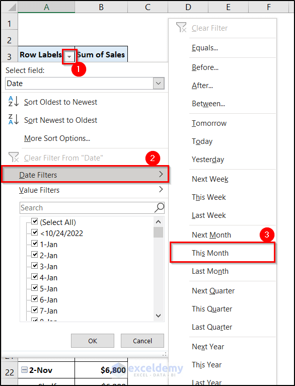
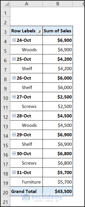
That’s it. Now you will see the pivot table contains a date filter that shows the data belonging to the current month.

If the month changes (the one in your operating system), the values that this Excel pivot table shows will also change.

Consequently, you will convert the text filter into a dynamic date filter in the Excel pivot table.

Download Practice Workbook

You can download the workbook used for the demonstration from the link below and try the methods yourself.

Conclusion

This was all about converting a text filter into a date filter in Excel’s different filter features. Hopefully, you can convert them to each other for your custom datasets. I hope you found this guide helpful and informative. If you have any questions or suggestions, let us know in the comments below.

<< Go Back to Filter in Excel | Learn Excel