How to Use Text Filter in Excel (5 Methods)

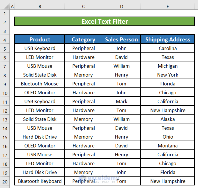
Dataset Overview

Let’s consider a scenario where we have an Excel worksheet containing information about products sold by a company to customers. The worksheet includes columns for Product Name, Product Category, Salesperson, and Shipping Address. Now, we’ll explore how to use the text filter in this Excel worksheet to filter text values.

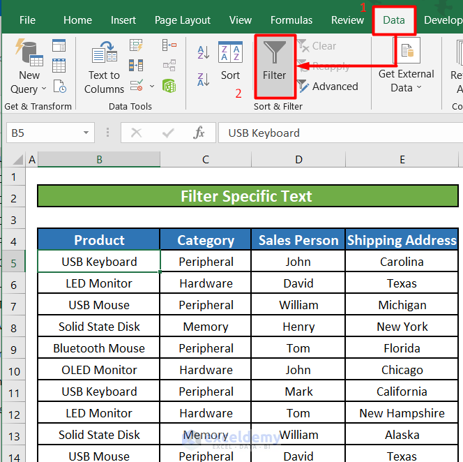
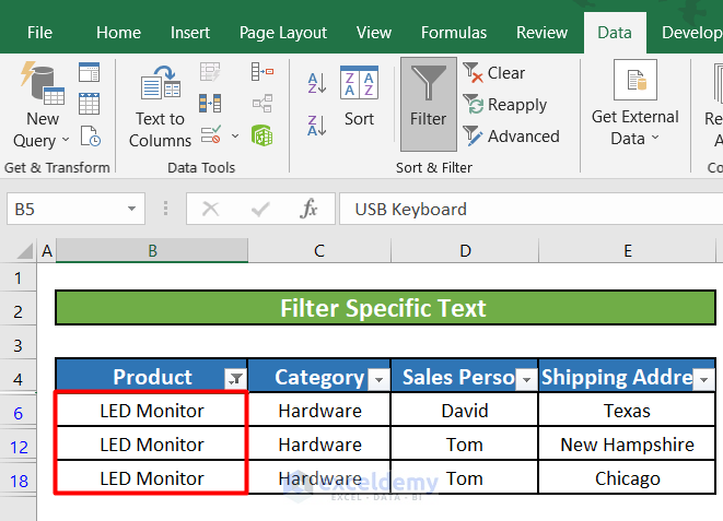
Method 1 – Apply Excel Filter to Filter Specific Text from the Worksheet

• Select a cell within your data range.
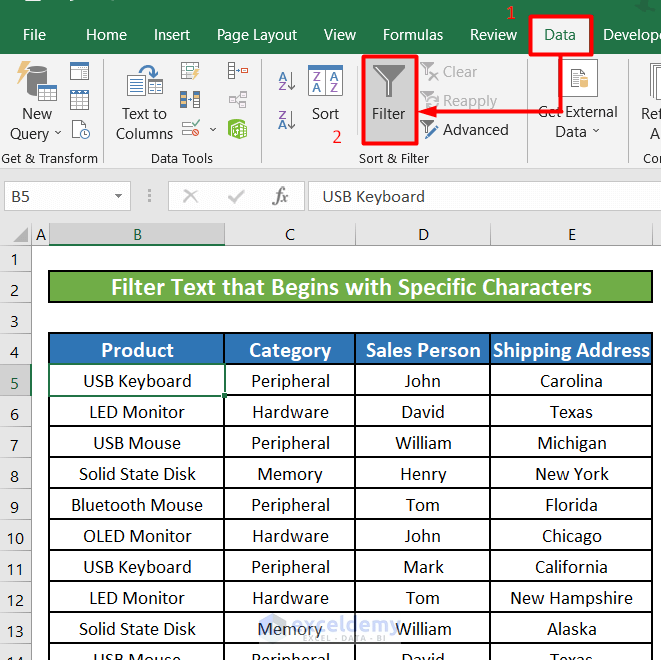
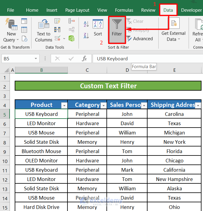
• Go to the Data tab.
• Click the Filter option in the Sort & Filter section.

• You’ll notice a small downward arrow at the bottom-right corner of each column header. Click the arrow next to the Product column.
• A window will appear with filtering options for the information in the Product column.

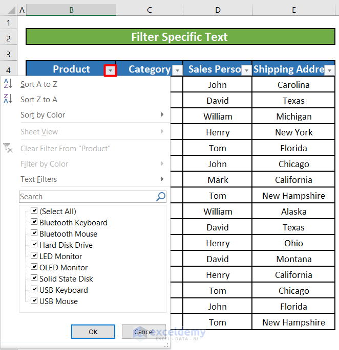
• Look for the Text Filters option. It lists the names of all unique products in the Product column, each with a select box next to it.
• Uncheck Select All and then choose only the LED Monitor option.
• Click OK.

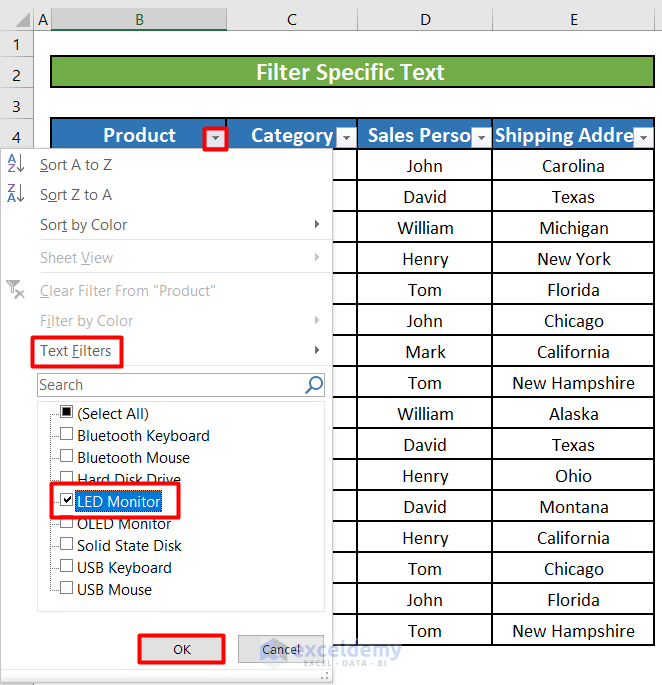
• The worksheet will now display only the rows where LED Monitor appears as a product.

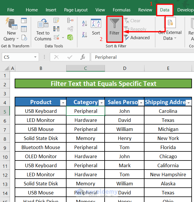
Method 2 – Use the Text Filter to Find Values that Equals Specific Text

We can also utilize the Excel text filter to identify values that equal or match a specific string of characters. In this example, we’ll filter all the rows where the product category is Memory using the Equals option of the text filter.

Steps:

• Apply filters to the columns in our worksheet:
  • Go to the Data tab.
  • Click on the Filter option.

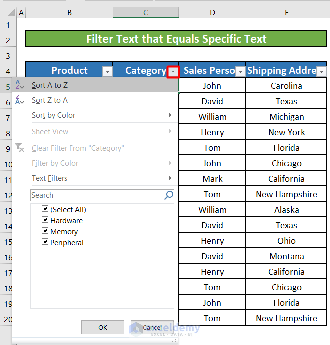
• After clicking the Filter option, you’ll notice a small downward arrow at the bottom-right corner of each column header. Click the arrow next to the Category column.
• A window will appear with options for filtering the information in the Category column. Look for the Text Filters option.

• Click on Text Filters, and another window will appear with various types of text filters.

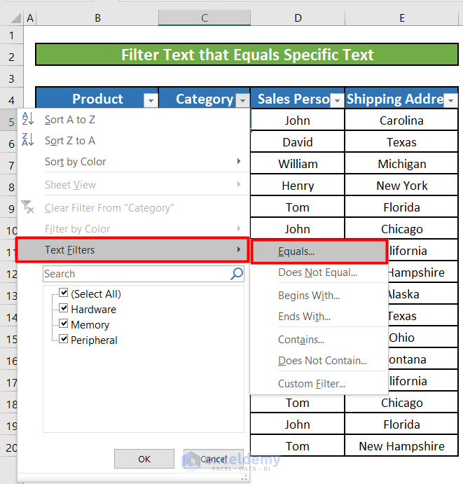
• In the Custom AutoFilter window that appears, there’s a drop-down menu to set the criteria for the Equals text filter. The default option is Equals, so leave it as is.

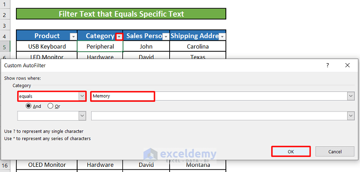
• Next to the drop-down menu, there’s an input box. Enter Memory in that box since we want rows that equal or match Memory as the category.
• Click OK.
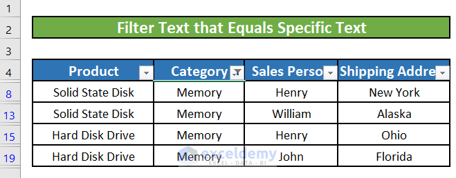
• Now your worksheet will display only those rows where the category is Memory.

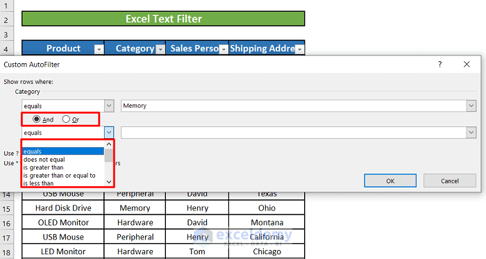
• You can also adjust the criteria for the Equals text filter. There are two options named And and Or just below the drop-down menu. Additionally, there’s another drop-down menu to set criteria for another Equals text filter. The results will vary based on the options selected from these menus, but it depends on whether you choose And or Or.

• For example, leave the option from the first drop-down (equals) unchanged.
• Selected Or.
• From the second drop-down, select equals and Hardware.
• Click OK.

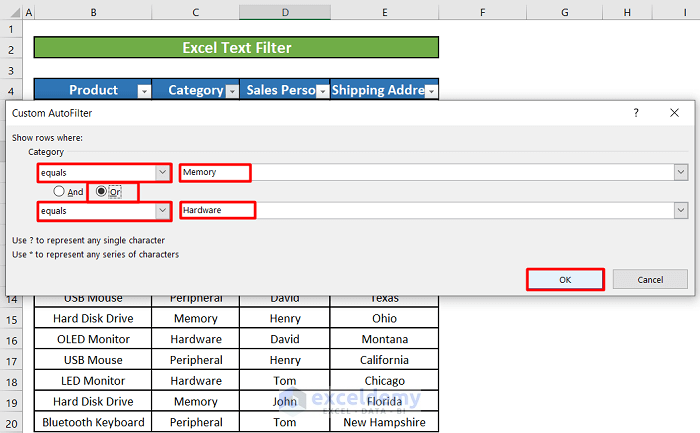
• Your worksheet now only has those rows that have Memory or Hardware as a product Category.

Method 3 – Apply the Text Filter to Find Texts that Begin with Specific Characters

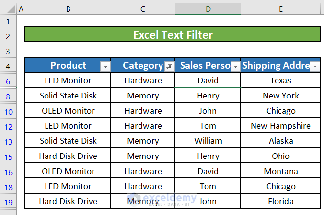
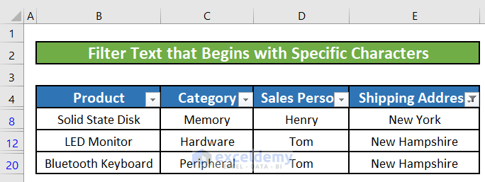
Another type of text filter allows us to filter rows based on text that begins with specific characters or a set of characters. For instance, we can filter rows where the shipping addresses start with New. This way, we’ll identify all rows with shipping addresses like New York or New Hampshire.

Steps:

• Apply filters to the columns in our worksheet:
  • Go to the Data tab.
  • Click on the Filter option.

• After clicking the Filter option, you’ll notice a small downward arrow at the bottom-right corner of each column header. Click the arrow next to the Shipping Address column.
• A window will appear with options for filtering the information in the Shipping Address column. Look for the Text Filters option.
• Click on Text Filters, and another window will appear with various types of text filters.

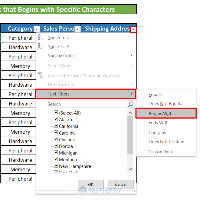
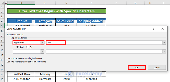
• In the Custom AutoFilter window that appears, there’s a drop-down menu to set the criteria for the Begins With text filter. The default option is Begins With, so leave it as is.
• Next to the drop-down menu, there’s an input box. Enter New in that box since we want rows with shipping addresses that begin with New.
• Click OK.

Your worksheet will display only the rows where the shipping addresses begin with New.

Similar to the Equals text filter, you can adjust the criteria for the Begins With filter. There are two options named And and Or just below the drop-down menu. Additionally, there’s another drop-down menu to set criteria for another Begins With text filter. The results will vary based on the options selected from these menus.

Method 4 – Use the Text Filter to Find Texts That Contain a Specific Set of Characters

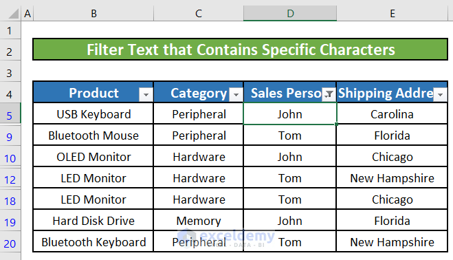
We can employ the text filter to identify rows containing a specific character or set of characters. For instance, let’s filter all the rows where the salespersons’ names have O as the second character.

Steps:

• Apply filters to the columns in our worksheet:
  • Go to the Data tab.
  • Click on the Filter option.

• After clicking the Filter option, you’ll notice a small downward arrow at the bottom-right corner of each column header. Click the arrow next to the Salesperson column.
• A window will appear with options for filtering the information in the Salesperson column. Look for the Text Filters option.
• Click on Text Filters, and another window will appear with various types of text filters.

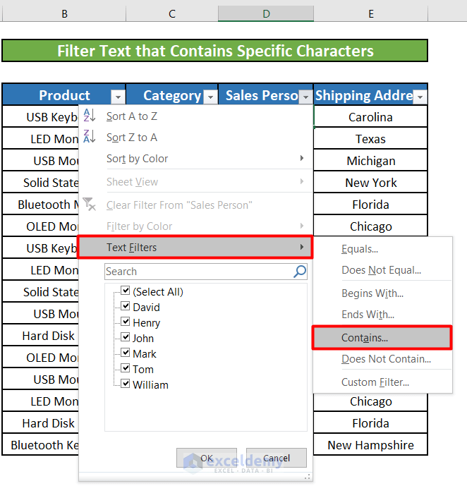
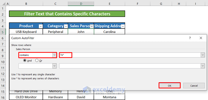
• In the Custom AutoFilter window that appears, there’s a drop-down menu to set the criteria for the Contains text filter. The default option is Contains, so leave it as is.
• Next to the drop-down menu, there’s an input box. Enter ?o* in that box. The question mark (?) before o will match only one character before o, and the asterisk (*) will match a series of characters or zero. This means the text filter will identify cells in the Salesperson column where the names have “o” as the second character, preceded by only one character. It can also contain a series of characters after the o.
• Click OK.

Your worksheet will display only the rows where the salespersons’ names have o as the second character.

Method 5 – Introduction to the Custom Text Filters in Excel

In addition to the predefined Text Filters, Excel offers a Custom Filter option that allows you to tailor your filtering criteria. With the Custom Filter, you can select different options from the text filter drop-down menus. Let’s explore how to use the Custom Filter to find shipping addresses that start with Ca.

 Steps:

• Apply filters to the columns in our worksheet:
  • Go to the Data tab.
  • Click on the Filter option.

• After clicking the Filter option, you’ll notice a small downward arrow at the bottom-right corner of each column header. Click the arrow next to the Shipping Address column.
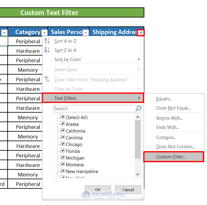
• A window will appear with options for filtering the information in the Shipping Address column. Look for the Text Filters option.
• Click on Text Filters, and another window will appear with various types of text filters.

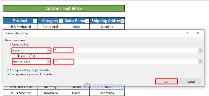
•  In the Custom AutoFilter window that appears, there are two drop-down menus (similar to what we’ve seen before) to set the criteria for the Custom Filter:
  • For the first drop-down menu, select equals and enter C in the input box next to it. This will find all shipping addresses that start with C.
  • For the second drop-down menu, select does not equal and enter ?h* in the input box next to it. This will exclude shipping addresses where the second character is h.
• Select the And option.
• Click OK.

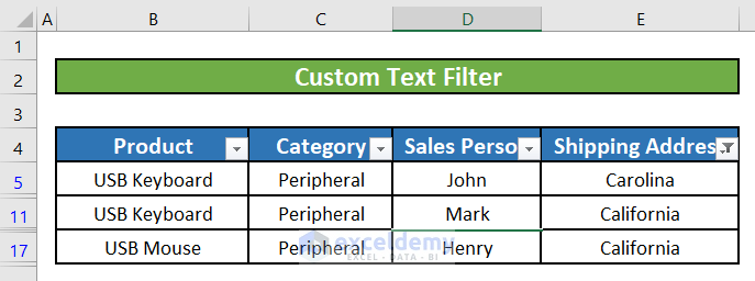
• Your worksheet will display only the rows where the shipping addresses start with “C” but do not have “h” as the second character – Carolina or California.

Things to Remember

• You can utilize additional text filters such as Does Not Equal, Ends With, and Does Not Contain. Does Not Equal” functions opposite to the Equals text filter. It eliminates or filters out values that match the provided text input.
• Ends With displays values that conclude with the specified character or characters provided in the filter. Does Not Contain reveals values that lack a specific character or set of characters. It removes values containing the character or characters specified in the filter.
• You can also use Does Not Equal, Ends With, Does Not Contain text filters.

Download Practice Workbook

You can download the practice workbook from here:

<< Go Back to Filter in Excel | Learn Excel