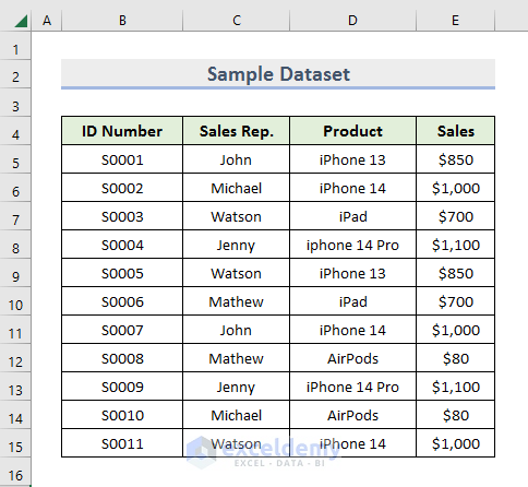
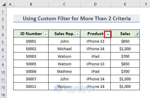
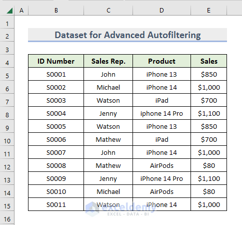
This is our sample dataset.
- We can use the Custom Autofilter to filter data with more than two criteria.
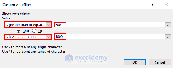
We will filter the records of iPhone 14 that have been sold at equal or greater than $500 as well as equal to or less than $1000.
- Click on the arrow sign in the Sales
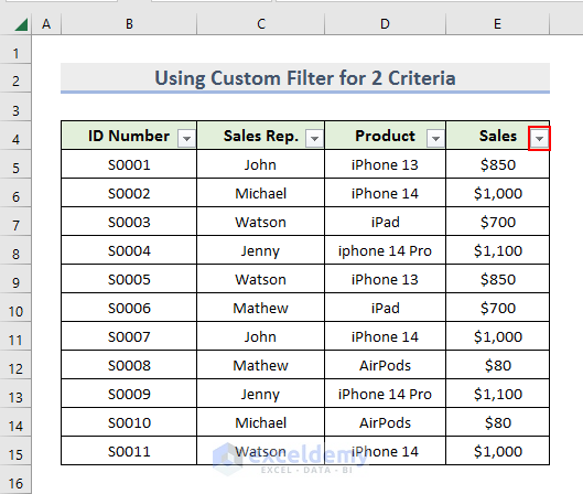
- From the Number Filters, select the Custom Filter
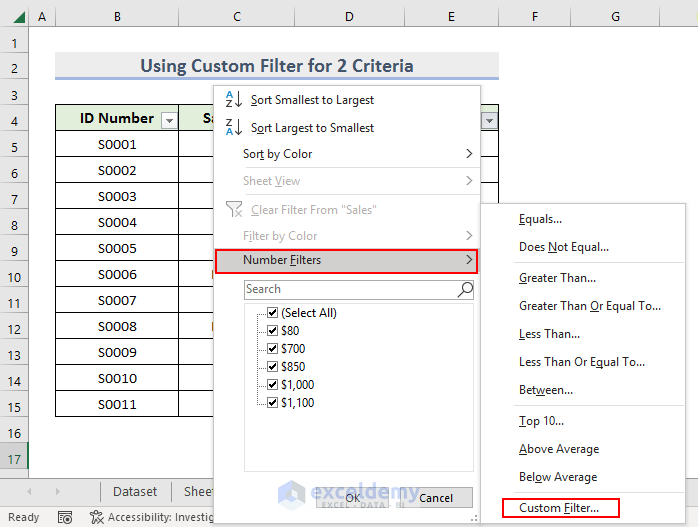
The Custom Autofilter window will open.
There are two criteria rows.
- In the first row, select is greater or equal to in the dropdown box and set 500 in the adjacent box.
- In the second row, select is less or equal to in the dropdown box and set 1000 in the adjacent box.
- Press OK.
The Sales that are between $500 and $1000 will be filtered and displayed in the Excel sheet.
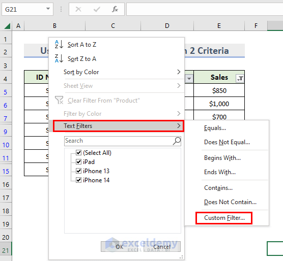
We will set another criterion. Suppose, we want to find out all the records of iPhone 14 which have been sold between $500 and $1000.
Click on the Arrowhead in the Product column.
In the pop-up window, go to the Text Filter option and Select Custom Filter.
- Select equals from the dropdown box and enter iPhone 14 in the adjacent box.
- Press OK.
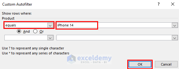
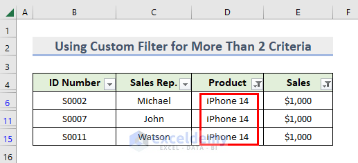
We will get results based on more than 2 criteria.
Using FILTER Function for More Than 2 Criteria
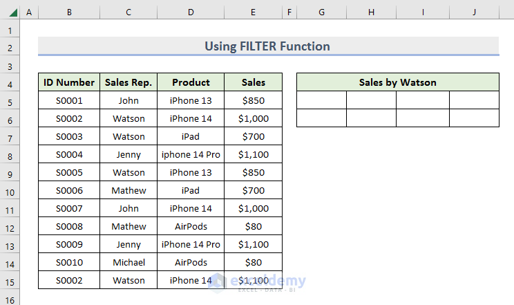
We can use the FILTER function to auto-filter with more than 2 criteria.
- For that, we have taken a dataset of sales reports of an Apple outlet. We want to find out the Sales by Watson with more than 2 criteria.
- Add another table as shown in the image below.
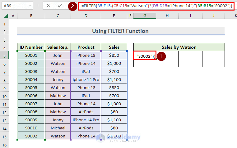
Add the following formula in G5:J6 and Press ENTER.
=FILTER(B5:E15,(C5:C15="Watson")*(D5:D15="iPhone 14")*(B5:B15="S0002"))
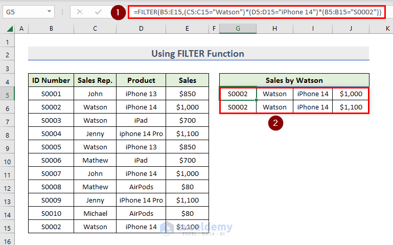
This formula returns results based on three criteria.
The range G5:J6 will show the result based on those three criteria.
Advanced Autofilter in Excel Using More Than 2 Criteria
In this process, we will create a data table. We have to set a criteria table and we will use the Advanced Filter tool to auto-filter the data table with more than 2 criteria.
- Create a data table. We have taken sample a data table containing information about the Sales report of an outlet of Apple.
This auto filter requires a criteria table.
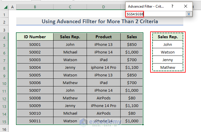
- We have added the single column Sales Rep. with 4 blank cells to set four criteria. You can set the criteria table according to your preference.
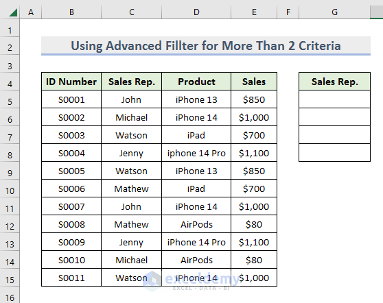
We want to filter the sales report of 4 Sale Reporters.
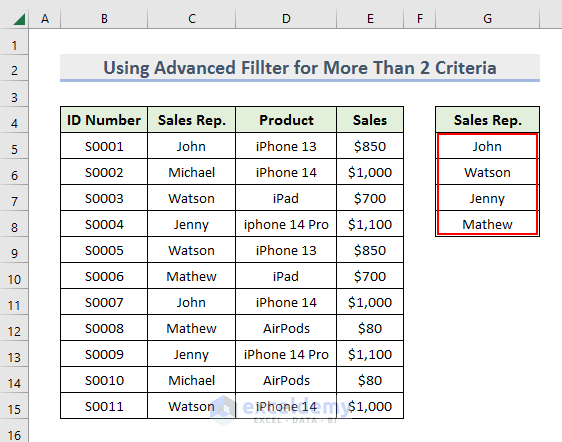
- Enter the names of Sales Reporters in the criteria table.
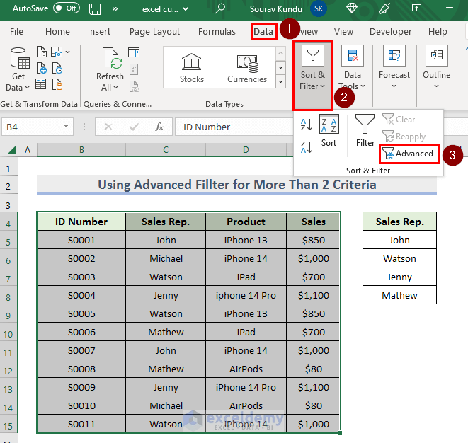
- Copy the data table B4:E15.
- Go to the Data ribbon and Select the Advanced filter option from the Sort & Filter section.
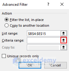
In the Advanced Filter window, you can see that the List range has already been selected.
- We have to set the criteria.
- Click on the Arrowhead in the Criteria range.
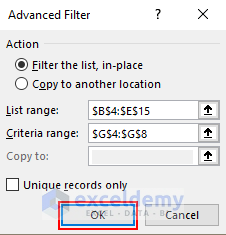
- Select the Criteria range as G4:G8 and click on the downward Arrowhead.
It will take you to the Advanced Filter window.
- Click on OK.
All the Sales records of the 4 sellers will be filtered out.
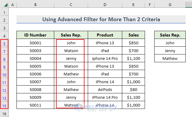
N.B: You can ignore the change in the criteria table.
Custom Autofilter in Excel Using Single Criteria
You can auto-filter the data set on a single criterion.
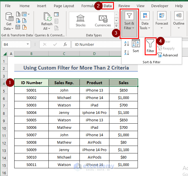
- Select your dataset.
- Go to the Data bar and select the Filter option from the Sort & Filter
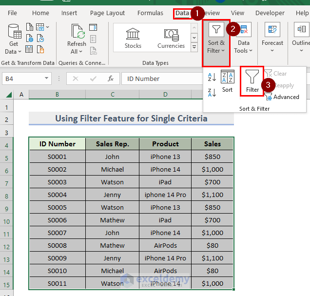
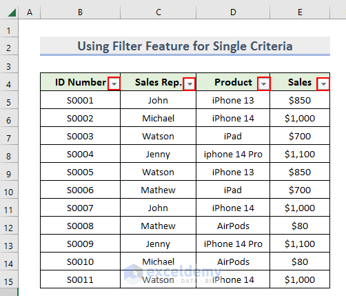
The Arrow sign will appear on table headings.
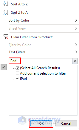
- We will set Product as the criteria. Click on the arrow in the Product heading.
- Enter the product name (ipad) in the Text Product box and press OK.
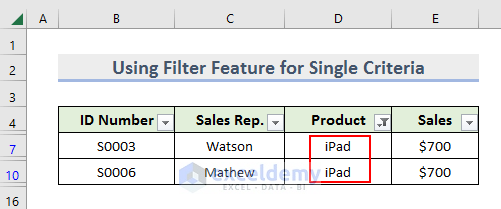
Records with the iPad will be filtered out and will be displayed in the spreadsheet.
Download Practice Workbook
<< Go Back to Excel Auto Filter | Filter in Excel | Learn Excel
Get FREE Advanced Excel Exercises with Solutions!

I have a list of warehouse bins that range from 099A to 15000F. When I use the Custom AutoFilter to only show bins that are in the 2000A range, I use “equals 20??A”
Problem is, there are locations that are named 200AA, 200BA, and 200CA. I need a way to filter the double letter bins out from this list without using a filter function that pulls the results into new cells. Something like “equals 20??A” and “does not equal *AA; *BA; *CA”
You know of a way to do this?
Hello Ryan,
To filter the double letter bins out from this list without using a filter function, see if using a range of characters works instead. Then, [0-9] should only match numeric characters. Follow the below steps:
1. Open the Custom AutoFilter dialog. (Read the article if necessary)
2. Enter Bin in Filed and type the below condition in Criteria:
20??[0-9][!A-Z]AHere,
– 20?? matches the first four characters (2000 to 2099).
– [0-9] matches the fifth character that it’s a numeric digit and not a letter.
– [!A-Z] matches any character that is not a letter from A to Z, effectively excluding double letters in the fifth and sixth positions.
– A matches the final “A” in the bin code.
As a result, the filter criteria will accurately find bins in the 2000A range that have a single numeric digit followed by a single letter “A” at the end, excluding those with double letters like 200AA, 200BA, and 200CA.
Regards,
Yousuf Khan Shovon