Latest Posts From Sourav Kundu

Dot Plot in Excel: Knowledge Hub How to Make a Dot Plot in Excel << Go Back To Excel Charts | Learn Excel

In this article, we will show you the different features of the Quick Analysis Tool in Excel. There are 5 core features of the Quick Analysis Tool. They are ...

How to Plot Line Graph with Single Line in Excel The sample dataset contains Sales by a company for the year 2018. Select the data range B5:C16. ...
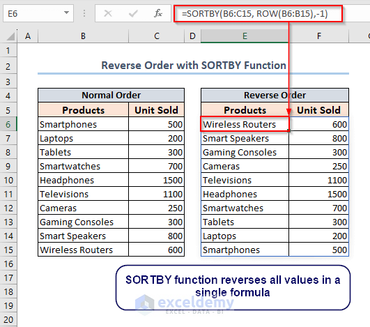
In this article, we will show you how to reverse order in Excel. We can reverse order vertically and horizontally in Excel. For this purpose, we can use the ...

How to Calculate Differentiation Manually in Excel? Steps: Set the differentiation equation. y= x2+7x+5 Dy/Dx = 2x+7 ...
This is an overview. Click the image for a detailed view Download Practice Workbook Recover Files.xlsx Method 1 - Recover Excel Files ...

Operators specify the type of calculation in an Excel formula. For example, arithmetic operators indicate addition, subtraction, multiplication, or division of ...

Edit Scatter Chart in Excel: Knowledge Hub How to Change Bubble Size in Scatter Plot in Excel How to Add Second Vertical Axis in Excel Scatter Plot ...
To generate the Mekko chart, we have taken the following dataset of different Markets and corresponding Company shares. Step 1 - Create Helper ...

In this article, you will learn to over 200+ shortcuts in Excel with practical examples. Click on the image to get a detailed view How Do I Read ...
Using Excel VBA, we can create a Digital Clock on a UserForm. This can be used as a visual reference for the current time, and to track the duration of the ...

The video below illustrates how to use Target Row to delete an entire row. By selecting Target Row, we have deleted all rows with marks less than 70 and no ...
![[Fixed!] Run Time Error 32809 in Excel VBA](https://www.exceldemy.com/wp-content/uploads/2023/05/run-time-error-32809-excel-vba10.png?v=1697520393)
The run time error 32809 in Excel VBA is quite complicated. Users often find this error irritating. For the same code, some devices will show the error and ...

Method 1 - Use of Ctrl + Pause Break Command to Pause and Resume Macro in Excel VBA We created this data table that will include the Sl. No. from B5 to ...

Step 1 - Define Names for the Dropdown List Create dropdown boxes for 3 different items: Month, Year, and Shift. Let's say we have five shifts ...
- 1
- 2
- 3
- 4
- Next Page »
See Our Reviews at


Hello, ALEJANDRO
Thank you for your comment. We have got an effective solution for your problem. We have taken 2 tables in the same worksheet as you can see from the following image:
To compare between these 2 tables, you can use the following VBA code:
Note: You should modify the Worksheet Name, Range and Cells references according to your data table.
When you run the VBA code, it will highlight the differences between the 2 tables in green color.
I hope, this is the solution you were looking for. If you have further queries let us know in the comment section. We will solve them as soon as possible.
Regards,
Sourav Kundu.
Exceldemy
Hi JOHN,
Thank you for sharing your problem with us. We have got a simple solution to your problem. You can use a VBA event for this purpose. Whenever you need a blank attendance sheet for a new month, you just have to change the value of the green-colored cell G5.
First, Right-click on your worksheet named Automated.
Then, click on View Code.
Then copy the following VBA code and paste it into the opening window:
Now, go back to the Automated sheet and insert Daily Attendences.
Now, write something in the G5 cell say N, and press Enter.
Instantaneously, the Automated sheet will be cleared and will create a new sheet Automated (2).
Now, go to the Automated (2) sheet and you can see the previous attendance record has been copied to this sheet.
The original worksheet is blank and is ready to take instructions from scratch.
Note: You can change the green color cell reference from the VBA code.
We hope that we have provided a reasonable solution to your problem. If you have more queries you can always mention them in the comment section.
Regards,
Sourav Kundu
Exceldemy.
Dear JOHN SINCLAIR,
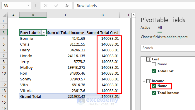
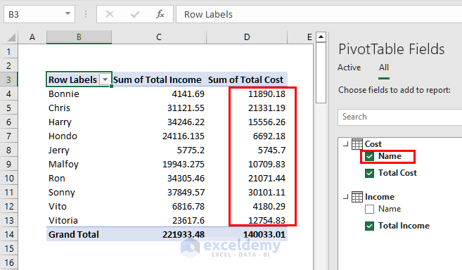
Thank you for sharing your problem with us. We have got a simple solution for your problem. It seems to us that you might be selecting the Name field from the Income table. That’s why Sum of Total Cost column is getting filled with 140033.01.
To solve this problem, make sure to mark the Name field from the Cost table and leave the Name field from the Income table unmarked. This will solve the problem and you will be able to merge different tables as you wanted.
We hope, our solution will work for your problem. If you face further difficulties with merging two pivot tables in Excel, you are always welcome to inform us.
Regards,
Sourav Kundu
Exceldemy
Hello SUNZEEV,
Thank you for your comment. Here, we are providing two revised formulas to meet your requirements.
For simplicity, we have modified the dataset with two additional Company names.
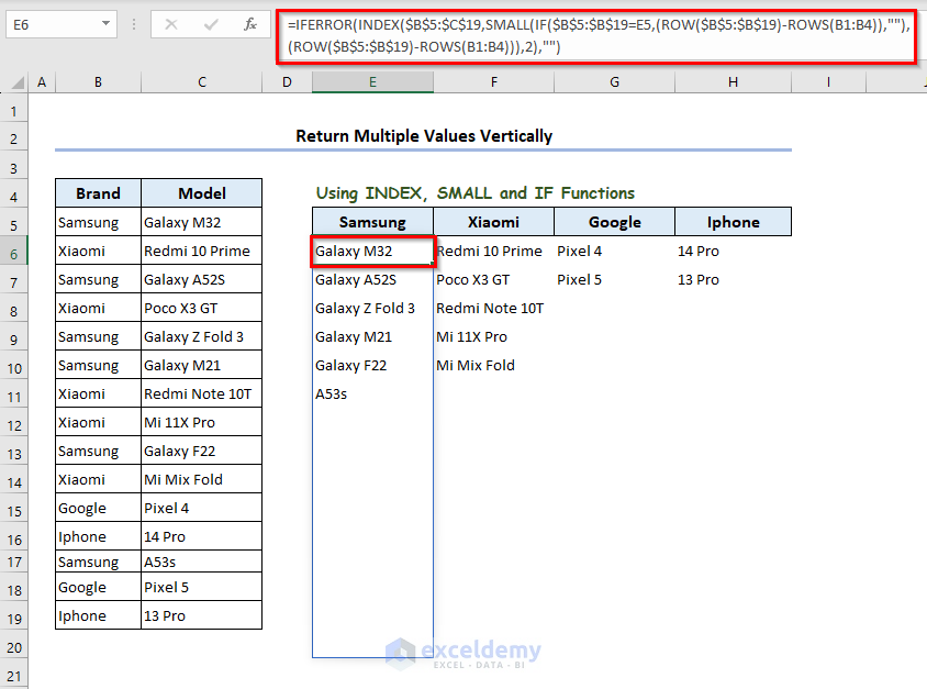
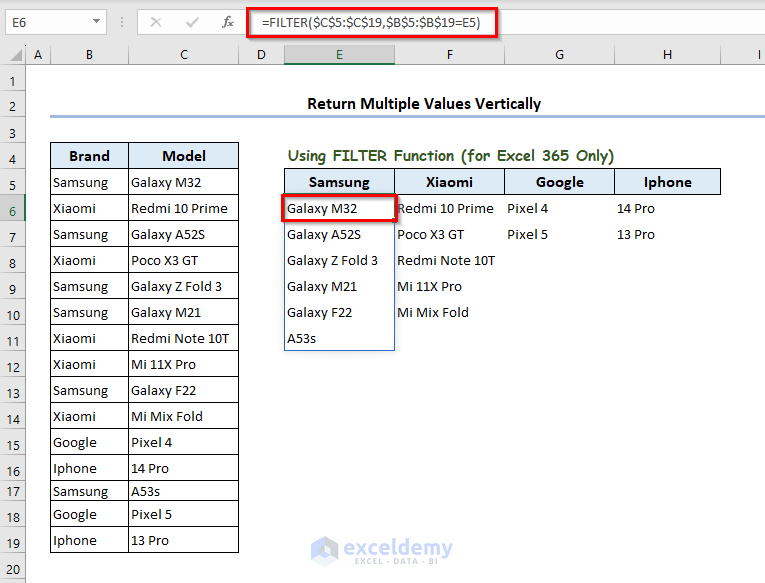
To get all the device names for each company, write the following formula in E6 and press Enter.
=IFERROR(INDEX($B$5:$C$19,SMALL(IF($B$5:$B$19=E5,(ROW($B$5:$B$19)-ROWS(B1:B4)),""),(ROW($B$5:$B$19)-ROWS(B1:B4))),2),"")You will get all the results of Samsung at once.
Now, drag the E6 cell to the right to H6 cell. You will get your desired results.
Another way is to use the FILTER function. For this method, write the following formula in E6 and press Enter.
=FILTER(C5:C19,B5:B19=E5)Now, drag the E6 cell to the right to the H6 cell. You will get your desired results. The FILTER function is available on Excel 365 only.
You can download the workbook from the link below.
Answer.xlsx
We hope these methods will satisfy your queries. If you have further questions, you are always welcome.
Regards,
Sourav
ExcelDemy.
Hi JEFF Z,
Thank you for sharing your problem with us. We have got a very simple solution to your problem. You just have to delete the last line (Call Shell(“TaskKill /F /IM Acrobat.exe”, vbHide)) from the code.
And, the revised code is given as follows:
The problem with the previous code was that the code would close the PDF file before pasting it into Excel. So, we have removed the last line so that, the code doesn’t close the pdf file at all. In this case, you have to close the pdf file manually.
Make sure to close the pdf file before running the code. And, also, make sure to clear the contents of Column 1 of Sheet 1 before running the code.
Regards,
Sourav Kundu
ExcelDemy.
Hi NN,
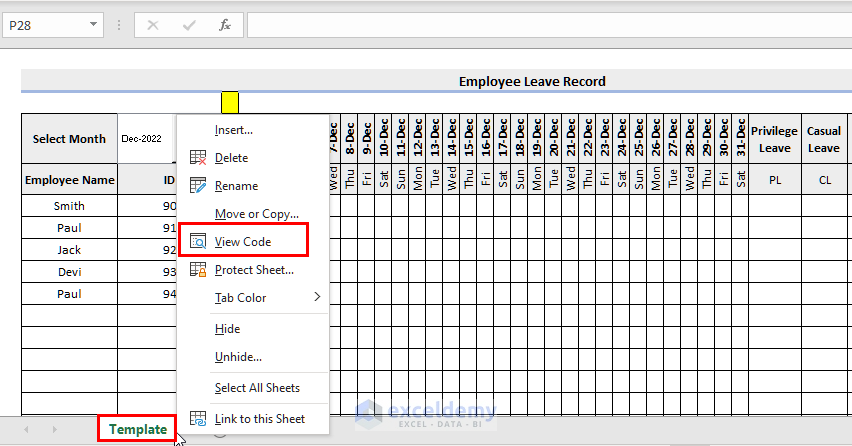
Thank you for sharing your problem with us. We have got a solution to your requirement. With this solution, whenever you need a blank record, you just have to change the value of the yellow-colored cell. You have to use a VBA code in the worksheet for the purpose.
First, Right-click on your worksheet named Template.
Then, click on View Code.
Then. copy the following VBA code and paste it into the opening window:
Now, go back to your workbook and insert some Employee Leaves.
Now, write something say N, and press Enter.
The code will create a new worksheet containing the Employee Leaves records.
Now, go back to the previous worksheet.
The original worksheet is blank and is ready to take instructions from scratch.
Note: You can change the Yellow color cell reference from the VBA code.
You can download the updated template with the VBA code from below:
Answer.xlsm
We hope that we have provided a reasonable solution to your problem. If you have more queries you can always mention them in the comment section.
Regards,
Sourav Kundu
Exceldemy.
Hello, STEVE C.
Thank you for sharing your problem with us. All the methods shown in the article should work perfectly for Microsoft 365 version. You might be using an older version. That’s why you are facing the problem. So, make sure to activate Microsoft 365 on your PC. Then, you should be able to use these procedures to get the color index.
Do let us know if your problem is solved or not.
Regards,
Sourav Kundu
ExcelDemy
Hello, RUSSEL.
Thank you for sharing your problem with us. We have provided 2 different ways to solve your problem.
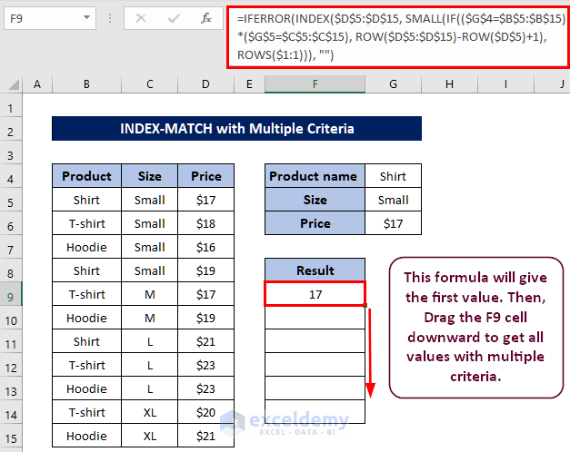
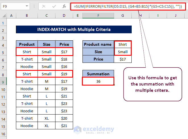
For example, we have a dataset of Product, Size, and Price. We will find the total price of the Small Shirts.
Method-1:
For this, write the following formula in the F9 cell and press Enter.
=IFERROR(INDEX($D$5:$D$15, SMALL(IF(($G$4=$B$5:$B$15)*($G$5=$C$5:$C$15), ROW($D$5:$D$15)-ROW($D$5)+1), ROWS($1:1))), "")And, you will get the first Price value.
Then Drag the F9 formula downwards to get other Price values that meet the criteria.
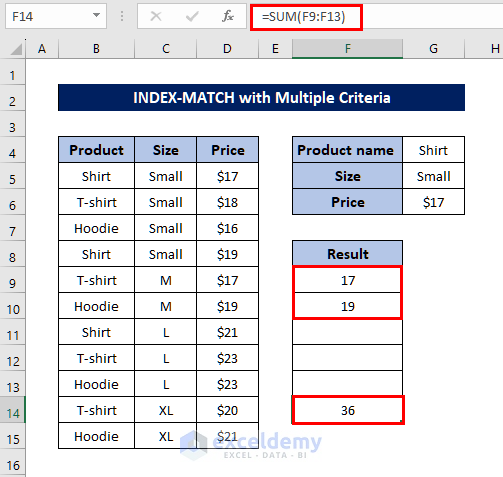
You can see that we have got two Price values that meet the multiple criteria.
Now, you can use the SUM function to get the total Price value.
Method 2:
Write the following formula in F9 and press Enter.
=SUM(IFERROR(FILTER(D5:D15, (G4=B5:B15)*(G5=C5:C15)), ""))And, you will get the total Price value with multiple criteria.
The FILTER function used in this method is only available for Microsoft 365 and Excel 2021.
Solution to Your Problem:
You can use the formula below to solve your problem:
=SUM(IFERROR(FILTER($G$20:$G$52, ($B$20:$B$53=$B3)*($E$20:$E$52=$D3)*($F$20:$F$52=CH$1)*($A$20:$A$53=$A3)*($D$20:$D$52=$E3)), ""))We could have given you the exact formula if we had your dataset. Let us know if your problem is solved.
Regards,
Sourav
ExcelDemy.
Hello, KENNY H.
Thank you for sharing your problem with us. However, we would have liked more information about your problem. The method described in this article should work perfectly. Try to follow the methods and steps given in this article as it is. Make sure to download the proper code 128 font.
You can email us screenshots of your problem or your workbook at [email protected]
That would really help us to understand your problem and give a proper solution.
You can also follow the articles below for generating barcodes in Excel.
1. Create Barcode in Excel
2. Generate 2D Barcode in Excel
Have a nice day!
Regards,
Sourav
Exceldemy.
Hi VIJAY,
Thank you for sharing your problem with us. As you wanted to determine each employee’s shift assuming that, their holiday can be any weekday, we have modified the attendance sheet. We hope this solution will meet your requirement.
1. First, you have to create a new table that will include the preferred work shifts of each employee.
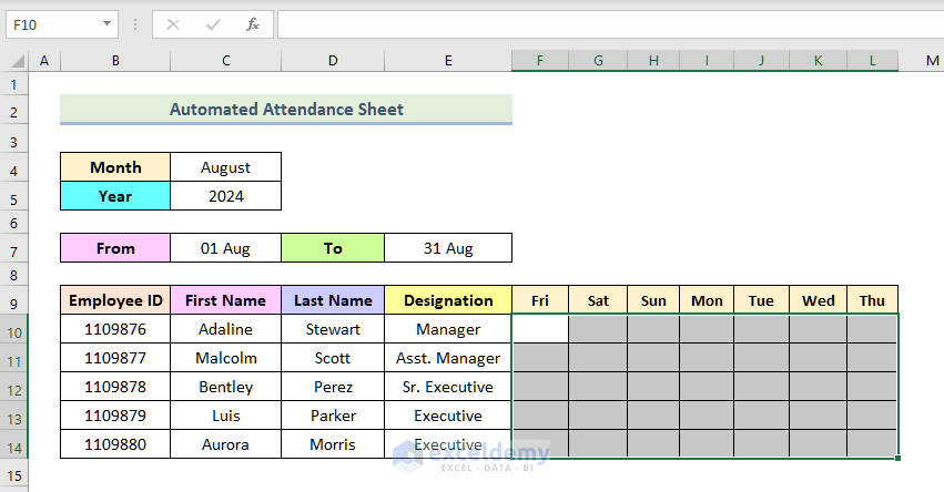

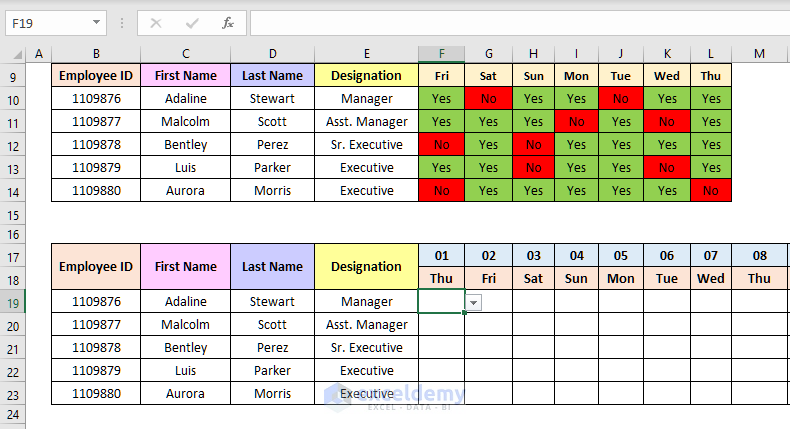
2. For simplicity, we are going to format these cells based on text value.
3. So, select the data range F10:L14.
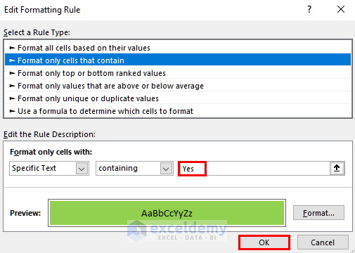
4. Now, from the Home tab go to Conditional Formatting and Select Format only cells that contain.
5. Then you have to set Yes as Specific Text.
6. Also, choose green as the format color.
7. Then, press the OK button.
8. Similarly, create another condition that if the cell contains the specific text No, the cell will be formatted as red.
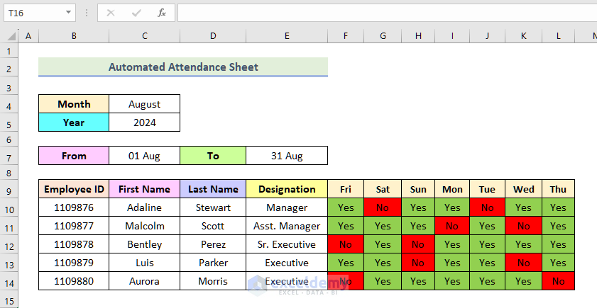
9. Your selected cells should still be blank.
10. Now, to indicate the work shift, write Yes or No in these formatted cells.
11. And, you can see the cells are instantaneously formatted with green and red colors (You can also use Yes or No from the drop-down box instead of writing them manually).
11. Now, go to the attendance sheet and suppose, there is no condition in this Shift table.
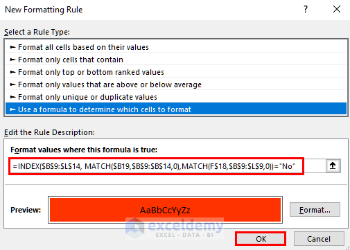
12. Select the F19 cell and create a new condition.
13. You have to select Use a formula to determine which cells to format as the New Formatting Rule.
14. Then, write the following formula in the formula box.
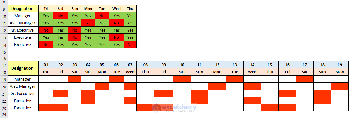
=INDEX($B$9:$L$14, MATCH($B19,$B$9:$B$14,0),MATCH(F$18,$B$9:$L$9,0))="No"15. Also, select a reddish format color and press OK.
16. Then, use the Fill Handle to copy the conditional formatting for all cells as shown in the following image.
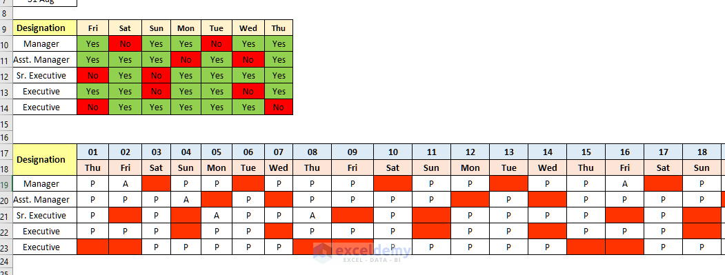
17. You can see, the Attendance table has been marked by each employee’s preferred off days.
18. Now, you can select Present (P) or Absent (A) for each employee.
You may need to modify the conditional format formula according to your data table. Be careful about relative and absolute referencing. You can also check the Excel file from the link below:
Answer.xlsx
We hope this comment has been useful to you. Have a nice day.
Regards
Sourav
Exceldemy.
Thank you MOhamad for your query. The Persian language is not available in the UNICODE. That’s why you are facing the problem. If you want to use the code for Persian characters, you have to modify the code slightly. The code can not take Persian language in the InputBox. So, instead of InputBox, we have to insert text to be highlighted in a cell. Let’s insert Persian text to be highlighted in the C10 cell. So, the modified vba code should be like this one.
Sub Text_Highlighter()
Application.ScreenUpdating = False
Dim Rng As Range
Dim cFnd As String
Dim xTmp As String
Dim x As Long
Dim m As Long
Dim y As Long
cFnd = Range(“C10”).Value
y = Len(cFnd)
Color_Code = Int(InputBox(“Enter the Color Code: ” + vbNewLine + “Enter 3 for Color Red.” + vbNewLine + “Enter 5 for Color Blue.” + vbNewLine + “Enter 6 for Color Yellow.” + vbNewLine + “Enter 10 for Color Green.”))
For Each Rng In Selection
With Rng
m = UBound(Split(Rng.Value, cFnd))
If m > 0 Then
xTmp = “”
For x = 0 To m – 1
xTmp = xTmp & Split(Rng.Value, cFnd)(x)
.Characters(Start:=Len(xTmp) + 1, Length:=y).Font.ColorIndex = Color_Code
xTmp = xTmp & cFnd
Next
End If
End With
Next Rng
Application.ScreenUpdating = True
End Sub
You should insert your preferred cell instead of C10. And this code will highlight characters of all other languages.
Hey Yann, we have tried your formula. But unfortunately, this formula is not working as you said it would. It gives a Value error instead.