This article will show you some methods to count unique values in an Excel worksheet based on different criteria. The Excel worksheet can count unique values, especially with multiple criteria. For a dataset, there can be unique values based on different criteria and we often need to count them.
How to Count Unique Values in Excel with Multiple Criteria: 3 Ways
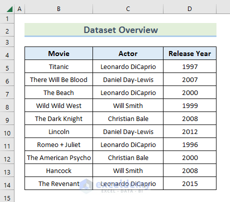
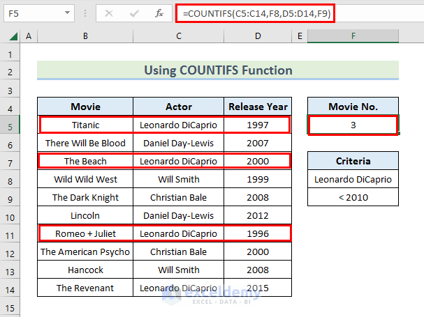
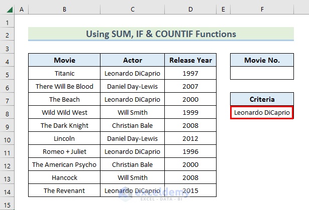
We have taken this dataset consisting of some great Movies, their Actors, and the Release Years. Let’s see how we can count the unique values based on multiple criteria using this dataset.
Method 1 – Using the COUNTIFS Function to Count Unique Values
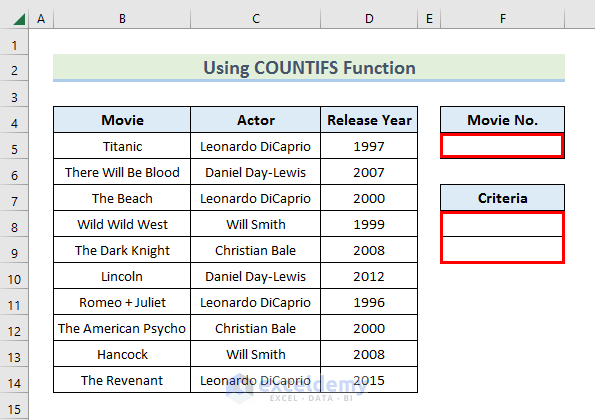
- We need a criteria table to set criteria.
- Allocate 2 cells where you have to insert criteria.
- Allocate another cell to insert the Formula.
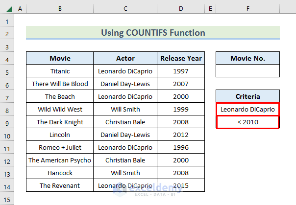
- We want to find out the number of movies with Leonardo DiCaprio and released before 2010.
- Write Leonardo DiCaprio in F8 and < 2010 in F9.
- Use the following formula in F5 and press Enter.
=COUNTIFS(C5:C14,F8,D5:D14,F9)
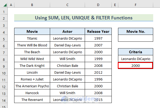
Method 2 – Combining SUM, LEN, UNIQUE, and FILTER Functions
We want to count the number of movies starring Leonardo DiCaprio before the year 2000.
- Write 2000 in F9.
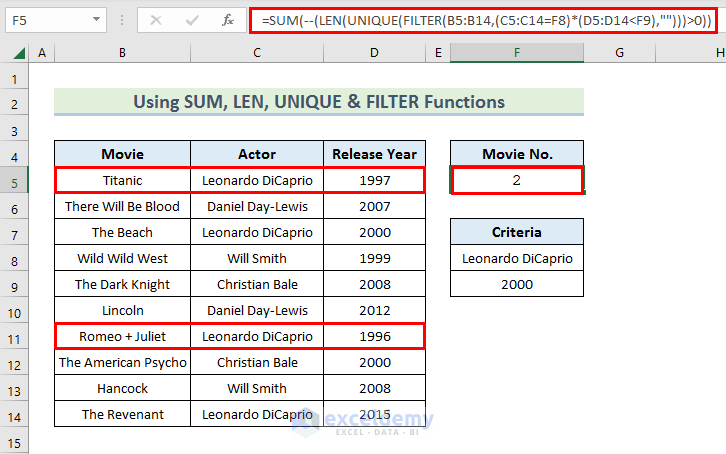
- Use the following formula in F5 and press Enter.
=SUM(--(LEN(UNIQUE(FILTER(B5:B14,(C5:C14=F8)*(D5:D14<F9),"")))>0))
Formula Breakdown
- FILTER(B5:B14,(C5:C14=F8)*(D5:D14<F9),””)): The FILTER Function extracts values from B5:B14 within the given criteria (C5:C14=F8) and (D5:D14<F9).
- Output: (Titanic, Romeo + Juliet)
- UNIQUE(FILTER(B5:B14,(C5:C14=F8)*(D5:D14<F9),””)): This UNIQUE Function returns the unique values.
- Output: (Titanic, Romeo + Juliet)
- LEN(UNIQUE(FILTER(B5:B14,(C5:C14=F8)*(D5:D14<F9),””)))>0): This LEN Function finds the length of each item and checks whether the value is greater than zero or not.
- Output: (1, 1)
- SUM(–(LEN(UNIQUE(FILTER(B5:B14,(C5:C14=F8)*(D5:D14<F9),””)))>0)): The SUM Function adds up the result.
- Output: (2)
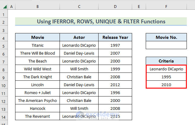
Method 3 – Merging IFERROR, ROWS, UNIQUE, and FILTER Functions
We want to count the number of movies starred by Leonardo DiCaprio between 1995 and 2010.
- Write these criteria in the criteria table.
- Use the following formula in F5 and press Enter.
=IFERROR(ROWS(UNIQUE(FILTER(B5:B14, (C5:C14=F8) * (D5:D14>F9)*(D5:D14<F10)))), 0)
We get 3 movies with Leonardo DiCaprio released between 1995 and 2010.

Formula Breakdown
- FILTER(B5:B14, (C5:C14=F8) * (D5:D14>F9)*(D5:D14<F10)): This FILTER Function finds values from the data range B5:B14 within the 3 given criteria.
- Output: (Titanic, The Beach, Romeo + Juliet)
- UNIQUE(FILTER(B5:B14, (C5:C14=F8) * (D5:D14>F9)*(D5:D14<F10))): The UNIQUE Function gives only the unique values from the data range.
- Output: (Titanic, The Beach, Romeo + Juliet)
- ROWS(UNIQUE(FILTER(B5:B14, (C5:C14=F8) * (D5:D14>F9)*(D5:D14<F10)))): The ROWS Function finds and returns the row numbers of a given array.
- Output: (5, 7, 11)
- IFERROR(ROWS(UNIQUE(FILTER(B5:B14, (C5:C14=F8) * (D5:D14>F9)*(D5:D14<F10)))), 0): This IFERROR Function returns some specified text in case of an error. Otherwise it returns the result.
- Output: (3)
Read More: How to Count Unique Text Values with Criteria in Excel
Counting Unique Values with Single Criteria
We want to find the number of movies with Leonardo DiCaprio.
- Write Leonardo DiCaprio in F8.
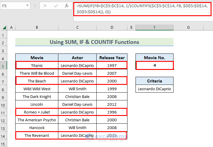
- Use the following formula in F5 and press Enter.
=SUM(IF(F8=$C$5:$C$14, 1/(COUNTIFS($C$5:$C$14, F8, $D$5:$D$14, $D$5:$D$14)), 0))
Formula Breakdown
- COUNTIFS($C$5:$C$14, F8, $D$5:$D$14, $D$5:$D$14): This COUNTIF Function counts all the values within given criteria but it doesn’t count the unique value.
- Output: (1,0,1,0,0,0,1,1,0,1)
- IF(F8=$C$5:$C$14, 1/(COUNTIFS($C$5:$C$14, F8, $D$5:$D$14, $D$5:$D$14)), 0): This IF Function returns 1 if the criteria is met. Otherwise, it gives 0.
- Output: (1,0,1,0,0,0,1,0,0,1)
- SUM(IF(F8=$C$5:$C$14, 1/(COUNTIFS($C$5:$C$14, F8, $D$5:$D$14, $D$5:$D$14)), 0)): This SUM Function adds all the values given in the range.
- Output: (4)
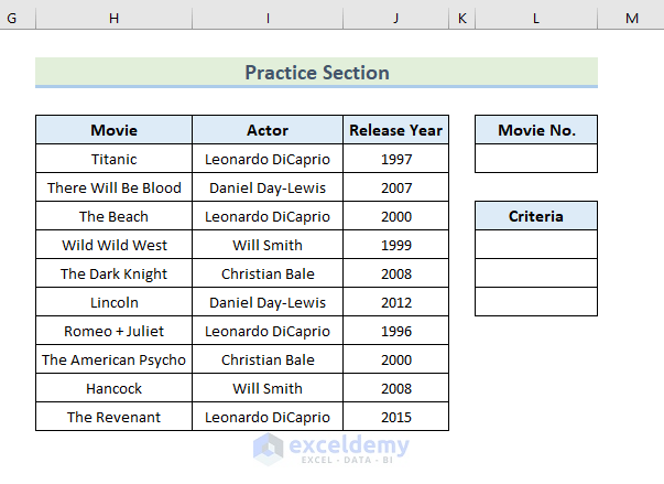
Practice Section
We have provided this practice section in the practice workbook which you can download and practice yourself.
Download the Practice Workbook
<< Go Back to Learn Excel
Get FREE Advanced Excel Exercises with Solutions!

Thank you so much.. it did helped me.. Love you
Hello Abishek,
You are most welcome.
Regards
ExcelDemy