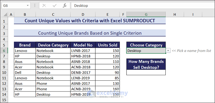
We have a dataset with Brand names, Device Categories, Model No, and Units Sold. We want to know how many brands (unique values) are selling notebooks (criteria) only.

Why Use SUMPRODUCT to Count Unique Values with Criteria?
You could use UNIQUE and FILTER functions instead of SUMPRODUCT. However, the UNIQUE function is not available in Excel before 2021. The FILTER function is available from Excel 2019.
So, if your Excel version is older than 2019, SUMPRODUCT can be a suitable option for you to count unique values based on conditions. SUMPRODUCT can return values based on criteria, but you have to combine COUNTIF or COUNITFS with it to count unique values.
Method 1 – Count Unique Values with a Single Criterion Using Excel SUMPRODUCT, IFERROR, and COUNTIFS Functions
Case 1.1 – Counting Unique Values with a Single Text Criterion
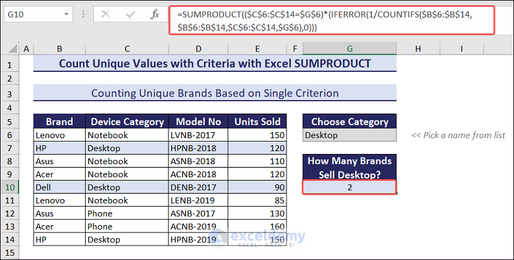
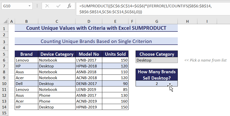
In cell G6, we specified a Device Category, for example, desktop. We are going to count the unique brand names that sell desktops in cell G10.
Follow these steps:
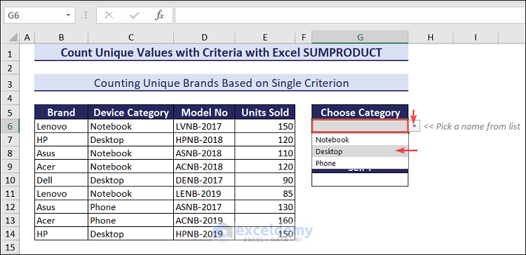
- Go to cell G6.
- Type desktop.
- We have created a drop-down list so that you can easily choose a category name from the list. Use that or type manually.
- Select cell G10 and insert the following formula:
=SUMPRODUCT(($C$6:$C$14=$G$6)*(IFERROR(1/COUNTIFS($B$6:$B$14,$B$6:$B$14,$C$6:$C$14,$G$6),0)))
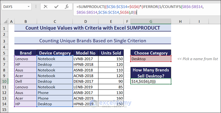
- Press the Enter key for the result.
- To know how many brands sell phones or notebooks, change the device category in cell G6 to phone or notebook, like the following GIF.
- We have applied the Conditional Formatting feature within the dataset so that the records can easily be noticed.
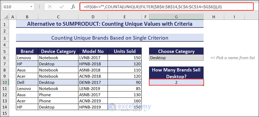
Easier Alternative Formula for Excel 2021 Users:
If you use Excel 2021 or Excel for 365, you can use the following formula.
=IF(G6<>"",COUNTA(UNIQUE(FILTER($B$6:$B$14,$C$6:$C$14=$G$6))),0)
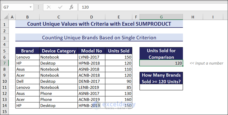
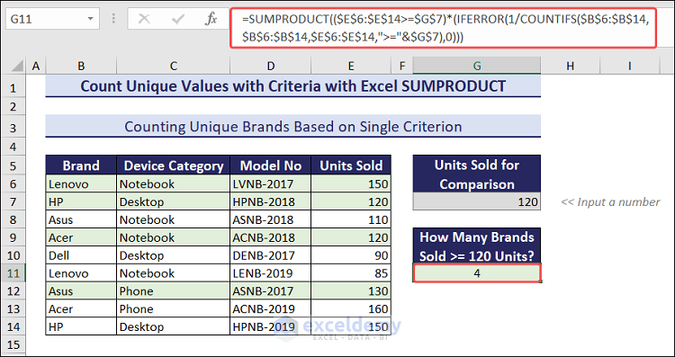
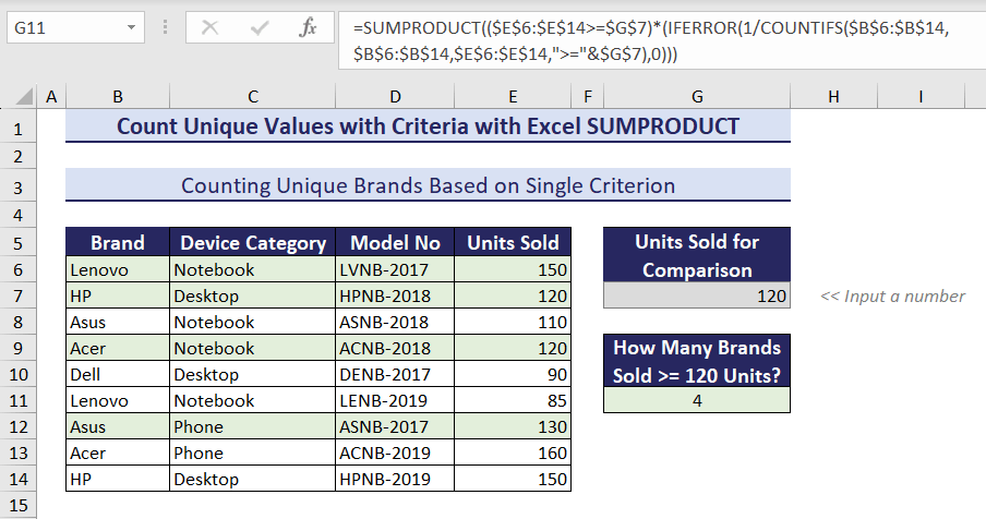
Case 1.2 – Counting Unique Values with a Single Number Criterion
We put a number in cell G7, for example, 120. In cell G10, we are going to count the unique brand names that sold at least 120 units of product.
Follow these steps:
- Go to cell G6.
- Type 120.
- Select cell G10.
- Insert the following formula.
=SUMPRODUCT(($E$6:$E$14>=$G$7)*(IFERROR(1/COUNTIFS($B$6:$B$14,$B$6:$B$14,$E$6:$E$14,">="&$G$7),0)))
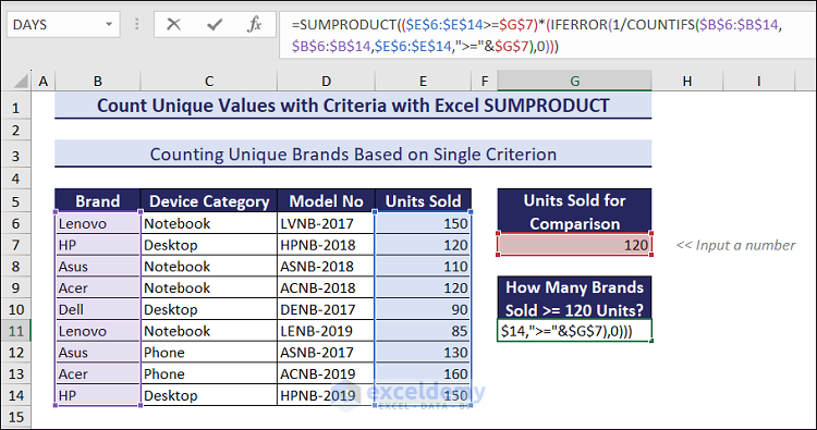
- Press the Enter key for the result.
- You can change the number in cell G6 for comparison, like the following GIF.
Note:
- If you want to apply other criteria operators to count unique values, change the operator inside the formula. For example, replace >= with < to apply “less than” criteria.
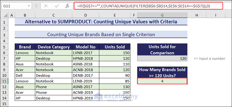
- If you use the Microsoft 365 or Excel 2021 version, you can use the following formula to count unique values based on the number criterion.
=IF($G$7<>"",COUNTA(UNIQUE(FILTER($B$6:$B$14,$E$6:$E$14>=$G$7))),0)
Method 2 – Count Unique Values with Multiple Criteria Using CEILING, SUMPRODUCT, IFERROR, and COUNTIF Functions
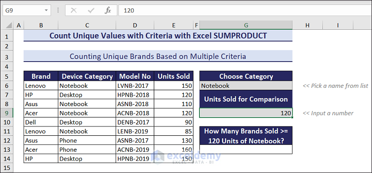
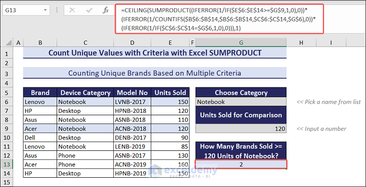
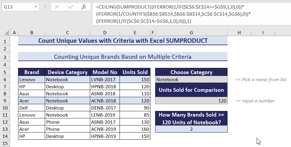
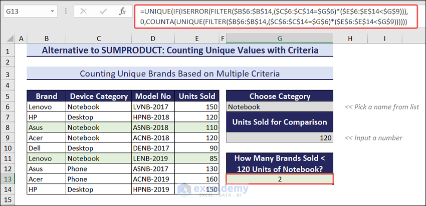
We’ll count how many brands have sold notebooks (criterion 1) and have sold at least 120 units (criterion 2).
Follow these steps:
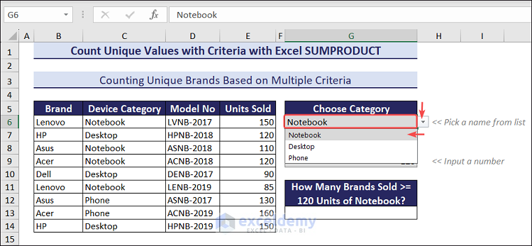
- Select cell G6.
- Choose Notebook as the category.
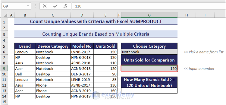
- Select cell G9.
- Type 120 as Units Sold for Comparison.
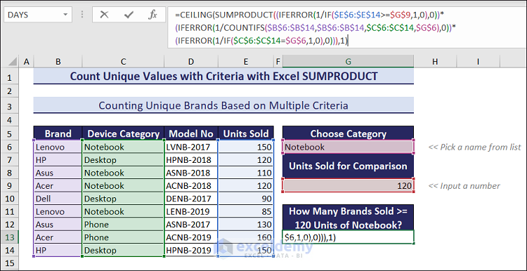
- Select cell G13.
- Insert the following formula.
=CEILING(SUMPRODUCT((IFERROR(1/IF($E$6:$E$14>=$G$9,1,0),0))*(IFERROR(1/COUNTIFS($B$6:$B$14,$B$6:$B$14,$C$6:$C$14,$G$6),0))*(IFERROR(1/IF($C$6:$C$14=$G$6,1,0),0))),1)
- Press Enter.
- You can also count unique brands by changing the device category and number of units sold.
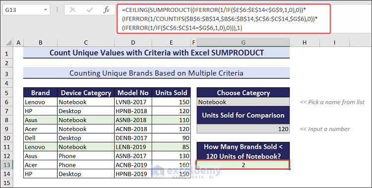
- To count the number of brands that sell notebooks and sales quantity less than 120, use the SUMPRODUCT formula:
=CEILING(SUMPRODUCT((IFERROR(1/IF($E$6:$E$14<$G$9,1,0),0))*(IFERROR(1/COUNTIFS($B$6:$B$14,$B$6:$B$14,$C$6:$C$14,$G$6),0))*(IFERROR(1/IF($C$6:$C$14=$G$6,1,0),0))),1)
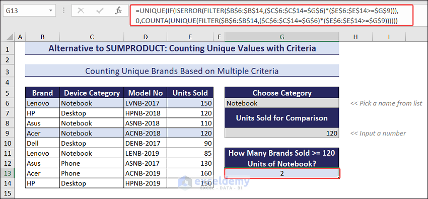
Alternative Formulas for Excel 2021 Users:
- For greater than or equal:
=UNIQUE(IF(ISERROR(FILTER($B$6:$B$14,($C$6:$C$14=$G$6)*($E$6:$E$14>=$G$9))),0,COUNTA(UNIQUE(FILTER($B$6:$B$14,($C$6:$C$14=$G$6)*($E$6:$E$14>=$G$9))))))
- For less than:
=UNIQUE(IF(ISERROR(FILTER($B$6:$B$14,($C$6:$C$14=$G$6)*($E$6:$E$14<$G$9))),0,COUNTA(UNIQUE(FILTER($B$6:$B$14,($C$6:$C$14=$G$6)*($E$6:$E$14<$G$9))))))
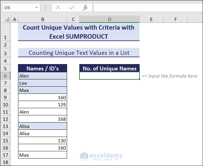
Method 3 – Count Unique Text Values Using ISTEXT and COUNTIF with SUMPRODUCT
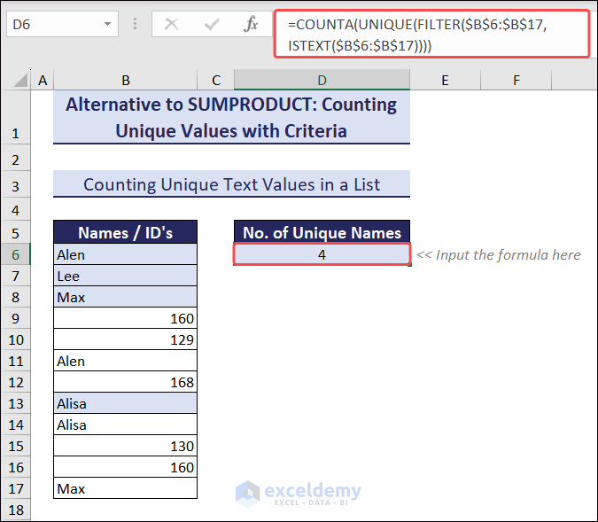
We have a dataset with a column titled Names / IDs like the following image. Under this column, there are some names and IDs in the range B6:B17. In cell D6, we will count the unique names, ignoring empty cells.
Follow these steps:
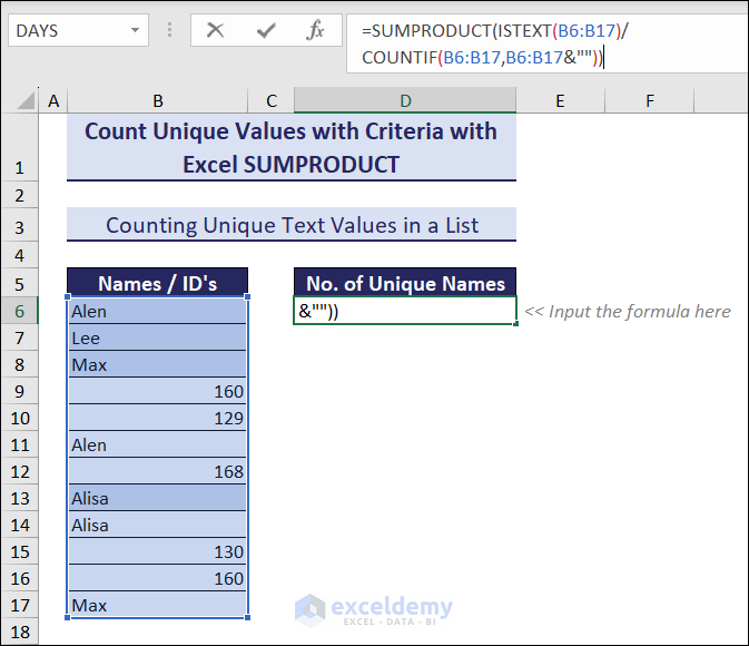
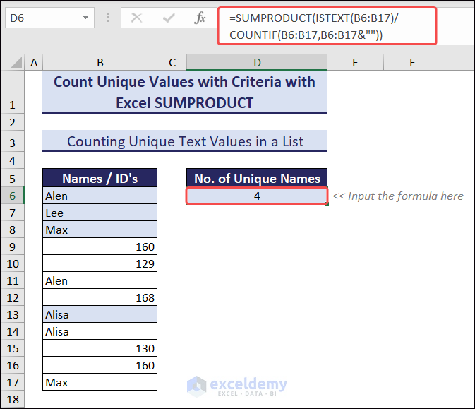
- Select cell D6 andinsert the following formula.
=SUMPRODUCT(ISTEXT(B6:B17)/COUNTIF(B6:B17,B6:B17&""))
- Press Enter.
Alternative Formula for Excel 2021 Users:
=COUNTA(UNIQUE(FILTER($B$6:$B$17,ISTEXT($B$6:$B$17))))
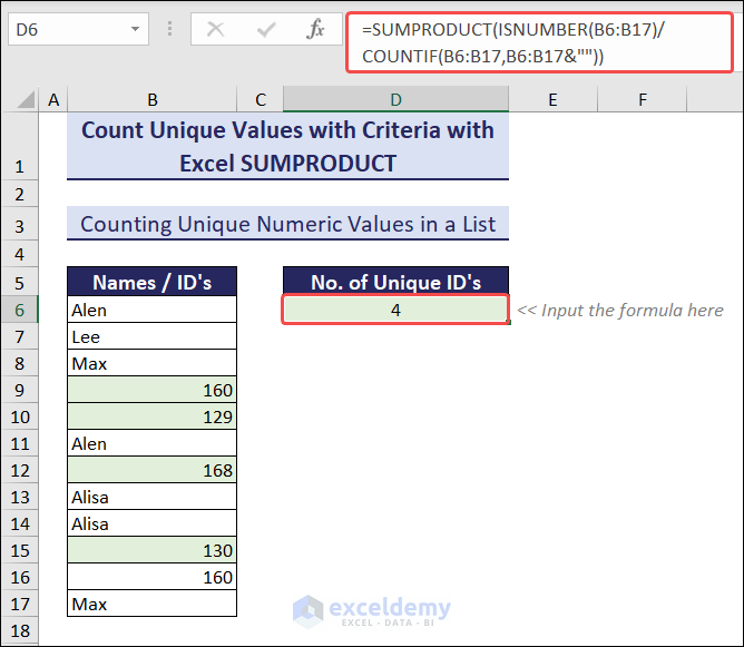
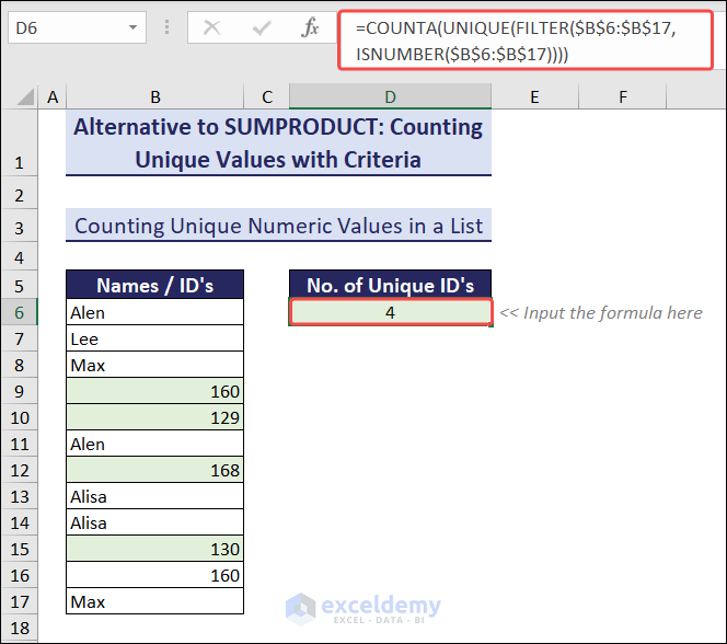
Method 4 – Count Unique Numbers Using ISNUMBER and COUNTIF with SUMPRODUCT
We will count the unique IDs that are in the number format, ignoring the empty cells within the range B6:B17.
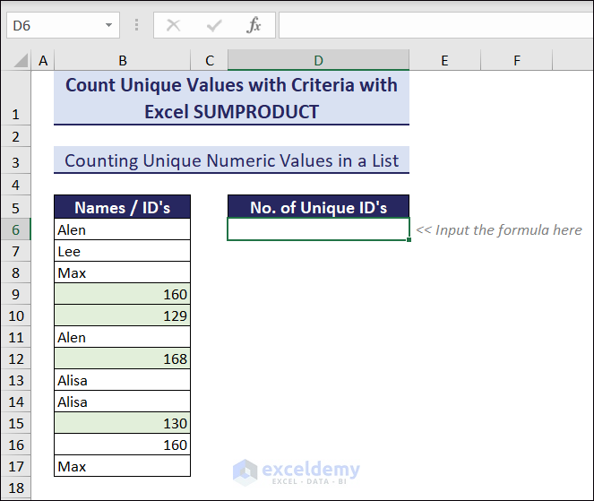
Follow these steps:
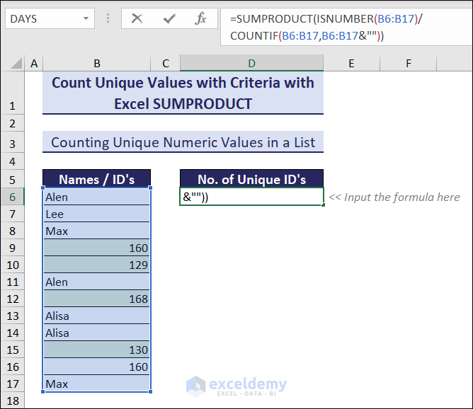
- Select the cell D6.
- Insert the following formula.
=SUMPRODUCT(ISNUMBER(B6:B17)/COUNTIF(B6:B17,B6:B17&""))
- Press Enter.
Alternative Formula for Excel 2021 Users:
=COUNTA(UNIQUE(FILTER($B$6:$B$17,ISNUMBER($B$6:$B$17))))
Download the Practice Workbook
<< Go Back to Learn Excel
Get FREE Advanced Excel Exercises with Solutions!
