How to Count Unique Values in a Filtered Column in Excel (5 Methods)

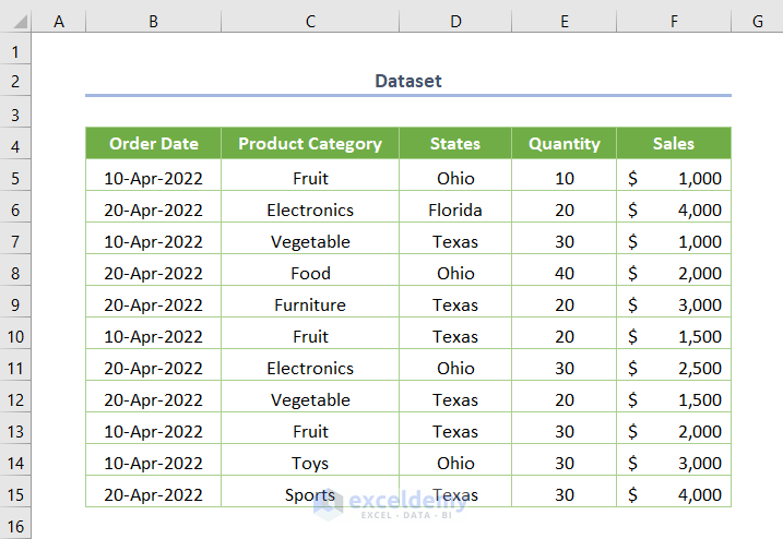
In today’s dataset, we have information on the Quantity and Sales of various Product Categories, along with Order Dates and corresponding States. Our task is to apply filters to specific columns and then count the unique values within those filtered columns.

Adding Filters

• Start by selecting the entire dataset where you want to apply filters.
• Go to the Sort & Filter ribbon in the Data tab.
• Click on the Filter tool to add filters to your dataset.

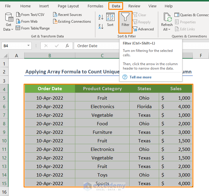
• Now, you’ll see a drop-down arrow next to each column header. Use these arrows to easily filter the data based on your criteria.

Method 1 – Using an Array Formula

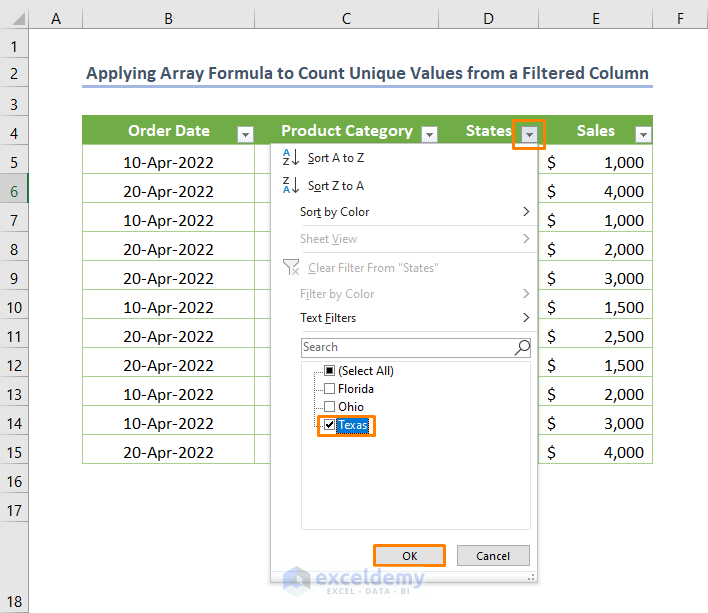
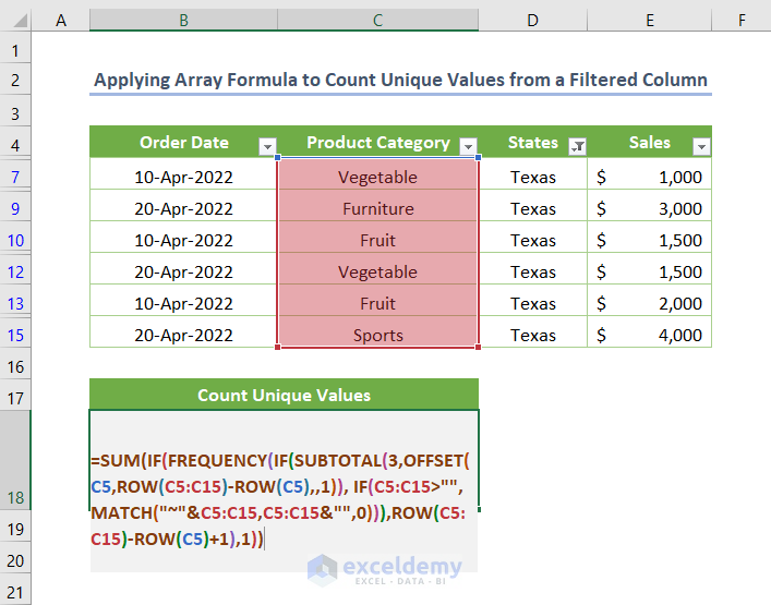
This method involves an array formula that may seem a bit complex but is quite handy. Suppose you want to filter the dataset based on Texas states.

Follow these steps:

• Click the drop-down arrow next to the States column header.
• Check the box for Texas to keep only the data related to that state.

• After applying the filter, you’ll have a filtered dataset.

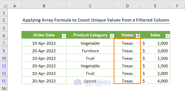
• To count the unique values in the Product Category column, insert the following array formula in cell B18:

• In this formula:
  • C5 represents the starting cell of the Product Category column.
  • C5:C15 is the cell range for that column.

Formula Breakdown:

In this formula, several functions work together to achieve the desired result. Let’s break it down step by step:

1. MATCH Function:
   • The MATCH function searches for specific values within a range and returns their relative positions.
   • In this case, it finds the values in the C5:C15 cell range (which represents the “Product Category” column) and returns an array of relative positions: {1,2,3,4,5,6,7,8,9,10,11}.
2. ROW Function:
   • The ROW function returns the row number of a given cell.
   • It’s used here to determine the row numbers within the C5:C15 range.
3. OFFSET Function:
   • The OFFSET function returns a reference to a cell or range based on a specified offset from a given starting point.
   • In this formula, it returns a reference to the cell specified by C5 (the starting cell of the “Product Category” column).
4. SUBTOTAL Function:
   • The SUBTOTAL function calculates a subtotal for a range of cells, considering only visible rows (i.e., rows that are not filtered out).
   • It’s used here to count the visible rows within the filtered dataset.
5. FREQUENCY Function:
   • The FREQUENCY function counts the unique values in a dataset.
   • It operates on the array of relative positions obtained from the MATCH function.
   • The IF function is used to ignore text and zero values.
6. SUM Function:
   • The SUM function aggregates the values returned by the FREQUENCY function.
   • It gives us the total count of unique values in the specified cell range.

Output

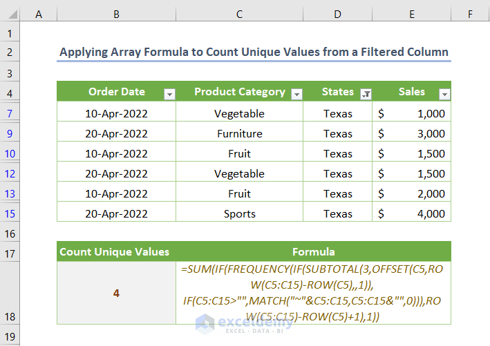
When you press ENTER after entering this formula, you’ll get the following output:

• The number of unique values is 4 because the two product categories (“Vegetable” and “Fruit”) have duplicates.

Note:

If you’re not using Microsoft 365, remember to press CTRL + SHIFT + ENTER when dealing with an array formula.

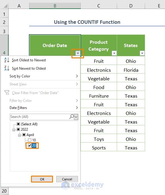
Method 2 – Using the COUNTIF Function

• Filtering the Dataset:
  • Before applying the COUNTIF function, let’s assume you want to filter the dataset based on the date 20-Apr-2022. Follow the same steps as in the first method to apply the filter.

• Applying the COUNTIF Function:
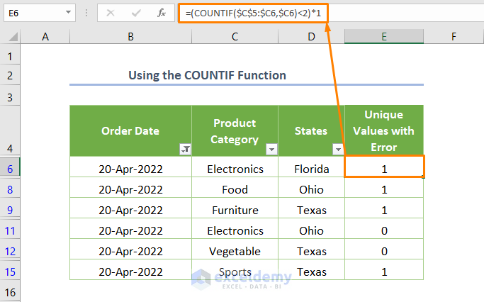
  • After filtering the entire dataset, you can use the COUNTIF function to count unique values within the filtered column.
  • The formula to achieve this is:

• • Here:
    • $C$5:$C6 represents the cell range of the Product Category column.
    • $C6 is the starting cell of the filtered field.
    • The COUNTIF function returns 1 for unique values and 0 for duplicate values.

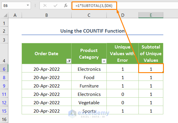
• Handling Errors:
  • If you closely examine the screenshot, you’ll notice an error in cell E12, where Vegetable shows 0 even though it is a unique category.

• • To address this, add a helper column to check visible rows using the SUBTOTAL function:

Here, $D6 is the output found using the COUNTIF function, and multiplying by 1 helps avoid issues with the last row in the filter range.

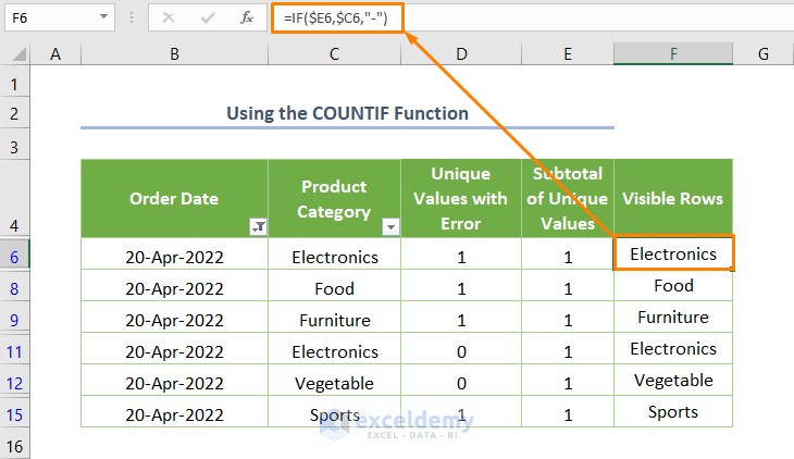
• Displaying Visible Rows:
  • Next, use the IF logical function to display visible rows:

• • • If $E6 (the starting cell of the output from the previous step) is true, it shows the corresponding value from column C; otherwise, it displays a hyphen (“-”) for hidden rows.

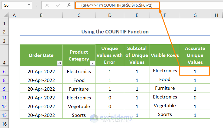
• Accurate Unique Values:
  • To obtain accurate unique values (excluding hidden rows), use the following formula:

• • • Here, $F6 is the starting cell of the output obtained earlier.

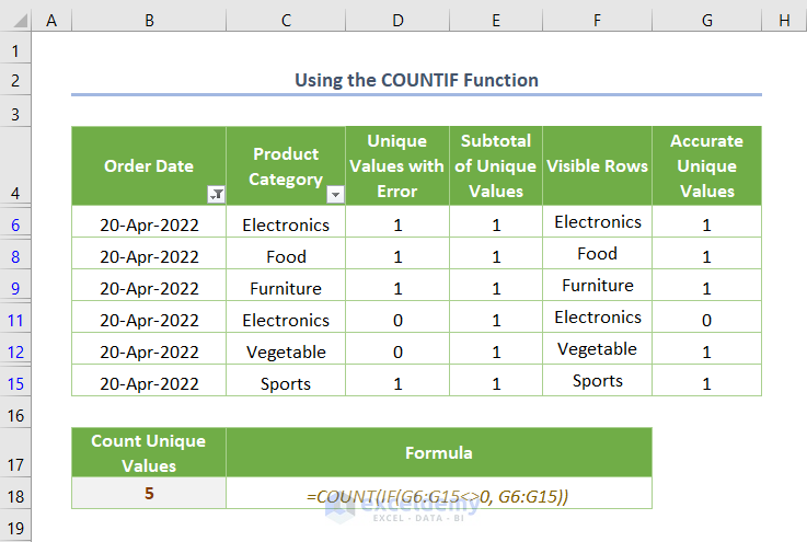
• Final COUNTIF Formula:
  • To count the unique values (excluding zero values), insert the following formula in cell B18:

• • • Here, G5:G15 represents the cell range of the Accurate Unique Values.

Method 3 – Combined Use of COUNTA, UNIQUE and FILTER Functions

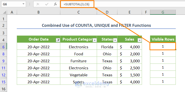
• Counting Visible Rows:
  • Before applying the combined formula, start by counting the visible rows using the SUBTOTAL function:

• • • Here, 3 corresponds to COUNTA, which counts cells including hidden rows, and C6 represents the starting cell of the filtered column.

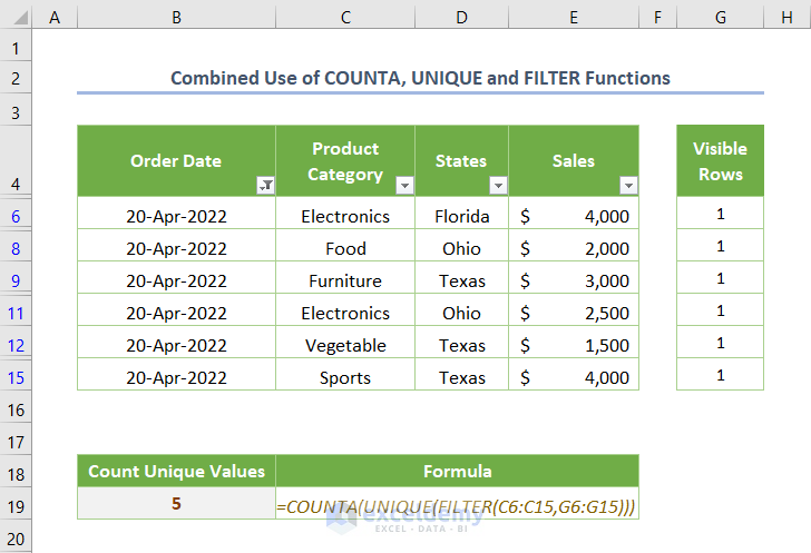
• Combined Formula:
  • Now, let’s insert the following combined formula to achieve our goal:

• • • In this formula:
      • C6:C15 represents the cell range of the Product Category column.
      • G6:G15 represents the cell range of the Visible Rows (filtered dataset).

• Function Breakdown:
  • The FILTER function filters the C6:C15 cell range based on the values in the G6:G15 cell range.
  • The UNIQUE function then identifies the unique values within the filtered data.
  • Finally, the COUNTA function counts all the filtered and unique values.

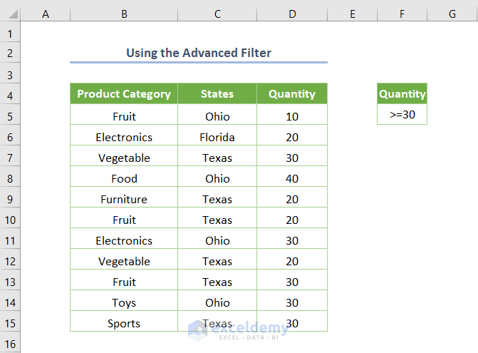
Method 4 – Counting Unique Values Using the Advanced Filter

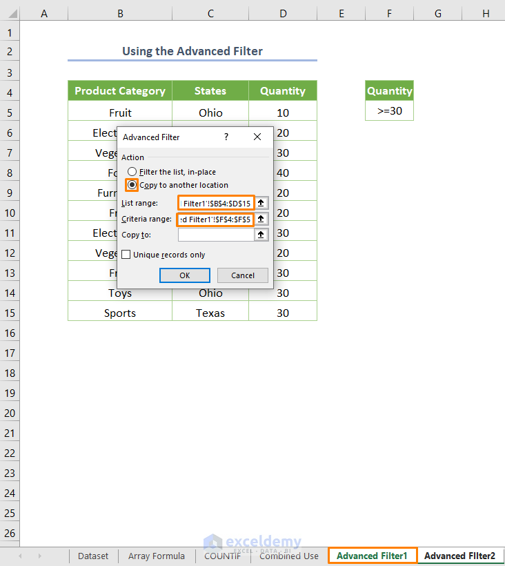
• Filtering Data Based on Quantity:
  • Suppose you want to filter data where the quantity is greater than or equal to 30 (cell range F4:F6).

• Creating a New Working Sheet:
  • To obtain the filtered unique data in a new working sheet, follow these steps:
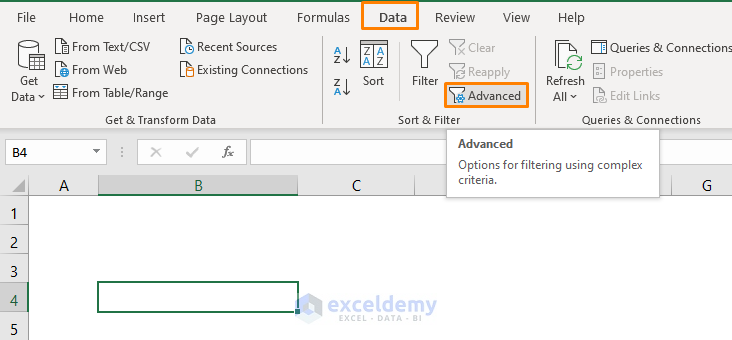
    • Create a new sheet.
    • Go to the Sort & Filter ribbon in the Data tab.
    • Choose the Advanced tool.

• Setting Up the Advanced Filter:
  • While keeping the cursor over the new working sheet (named Advanced Filter2):
    • Specify the List range as Advanced Filter1′!$B$4:$D$15.
    • Set the Criteria range as ‘Advanced Filter1’!$F$4:$F$5.
    • Before proceeding, check the circle next to the Copy to another location option.

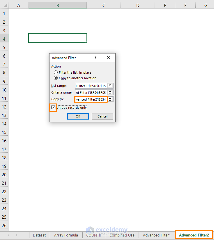
• • • Note: Advanced Filter1 refers to the existing working sheet, and Advanced Filter2 is the name of the new working sheet.

• Copying Unique Records:
  • Next, specify ‘Advanced FIlter2’!$B$4 after the “Copy to” option.
  • Check the box for Unique records only.
  • Press OK.

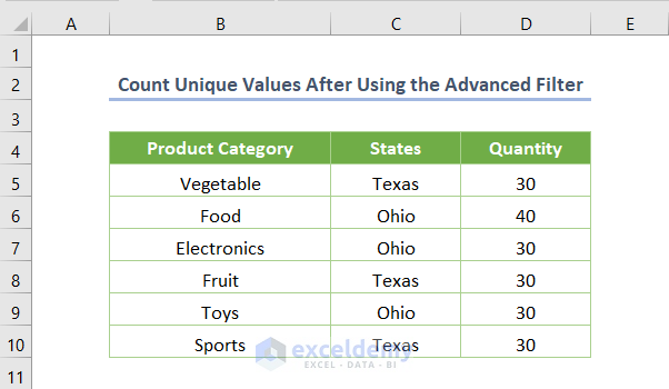
• Result:
  • After completing these steps, you’ll have a filtered dataset containing unique records.

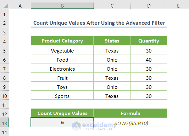
• Counting Unique Values:
  • To count the unique values, simply use the ROWS function with the following formula:

• • • Here, B5:B10 represents the cell range for the filtered Product Category.

Method 5 – Using the Pivot Table to Count Unique Values in Filtered Column

In addition to the four previously mentioned methods, you can utilize the Pivot Table—a powerful feature in Excel—to efficiently analyze larger datasets. Creating a Pivot Table is straightforward:

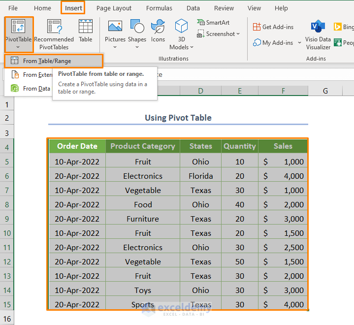
• Select the Entire Dataset: Choose the entire dataset you want to analyze.
• Insert a Pivot Table: Go to the Insert tab and select Pivot Table from the options.

• Configure the Pivot Table:
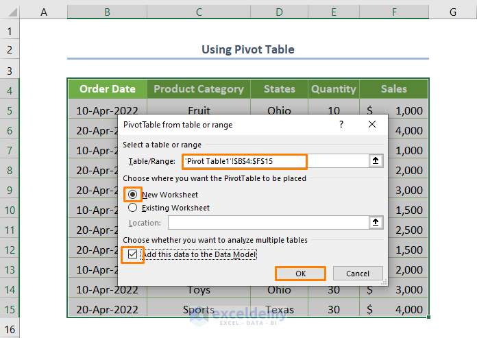
  • Check the box for New Worksheet to create the Pivot Table on a new sheet.
  • Optionally, select Add this data to the Data Model.

• Arrange Fields:
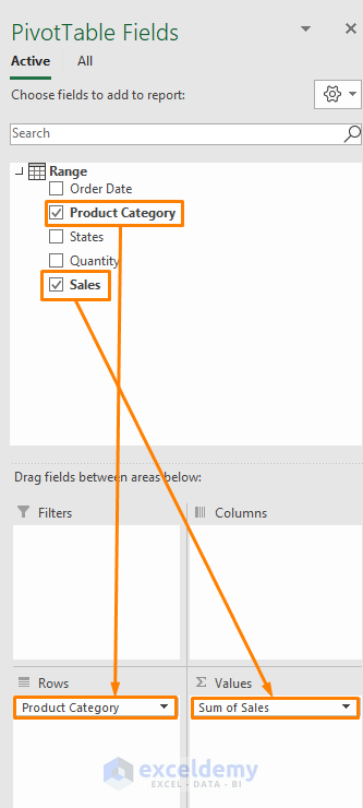
  • Place the Product Category field in the Rows area.
  • Put the Sales field in the Values area.

• Customize the Count:
  • Right-click on a cell in Column B.
  • Choose Value Field Settings.

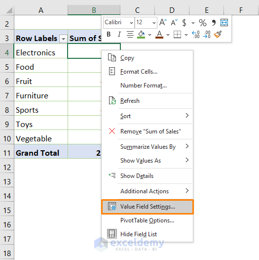
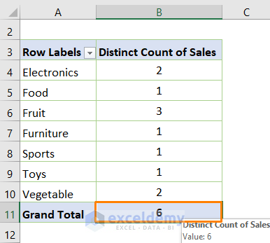
• • Select Distinct Count as shown in the image below.

• View the Result:
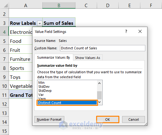
  • The output will display the number of unique values (in this case, 6).

Download Practice Workbook

You can download the practice workbook from here:

<< Go Back to Count | Unique Values | Learn Excel