The COUNTIFS Function
The COUNTIFS function counts the number of cells in a range that match one of the provided conditions.
- Syntax
COUNTIFS (range1, criteria1, [range2], [criteria2], …)

- Arguments
range1: [required] This is the first range to be evaluated.
criteria1: [required] range1 criteria.
range2: [optional] This is the second range to be evaluated.
criteria2: [optional] range2 criteria.
- Return Value
The total number of times a set of criteria is met.
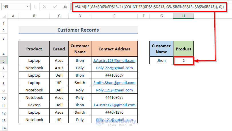
The dataset contains Product names in column B, the Brand in column C, Customers’ names in column D, and the Contact Address for each customer in column E. 
Example 1 – Estimate Unique Values Based on a single Criterion in Excel
STEPS:
- Select the cell in which you want to count the unique values. Here, H5.
- Enter the formula.
=SUM(IF(G5=$D$5:$D$13, 1/(COUNTIFS($D$5:$D$13, G5, $B$5:$B$13, $B$5:$B$13)), 0))- Press Enter to see the result.
Formula Breakdown
G5=$D$5:$D$13: finds the cells containing Jhon. Here, G5.
COUNTIFS($D$5:$D$13, G5, $B$5:$B$13, $B$5:$B$13: returns TRUE for addresses occurring once only; for repeated addresses. returns FALSE.
1/(COUNTIFS($D$5:$D$13, G5, $B$5:$B$13, $B$5:$B$13): divides the formula by 1 and returns 0.5.
IF(G5=$D$5:$D$13, 1/(COUNTIFS($D$5:$D$13, G5, $B$5:$B$13, $B$5:$B$13)), 0): checks whether the conditions in the formula are met and returns 1. 0, otherwise.
SUM(IF(G5=$D$5:$D$13, 1/(COUNTIFS($D$5:$D$13, G5, $B$5:$B$13, $B$5:$B$13)), 0)): counts the total unique values.
Example 2 – Multiple Criteria to Count Unique Excel Values
STEPS:
- Select the cell in which you want the result. Here, I5.
- Enter the formula.
=COUNTIFS(D5:D13,G5,C5:C13,H5)- Press Enter.
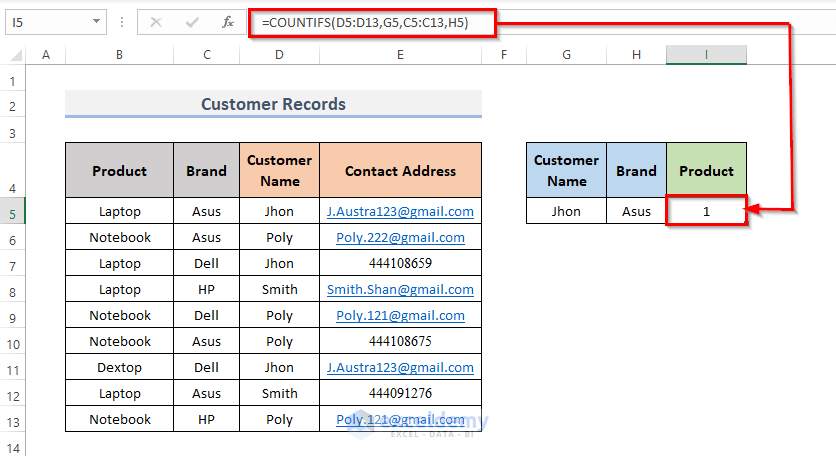
D5:D13 indicates the Customer Name, and the criteria for this range is G5 (Jhon).
C5:C13 indicates the Brand, and the criteria for this range is H5 (Asus).
Read More: How to Count Unique Names in Excel
Example 3 – Counting Different Number of Text Values in Excel
STEPS:
- Select the cell in which you want to count the unique values using the criteria. Here, G5.
- Enter the formula.
=SUM(--(ISTEXT(E5:E13)*COUNTIFS(E5:E13,E5:E13)=1))- Press Enter.
There are 2 unique text values.
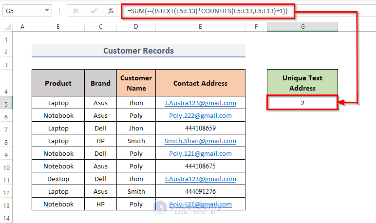
Formula Breakdown
ISTEXT(E5:E13): returns TRUE for all addresses that are text values. FALSE, otherwise.
COUNTIFS(E5:E13,E5:E13): returns TRUE for all addresses that appear just once and FALSE for all addresses that appear more than once.
ISTEXT(E5:E13)*COUNTIFS(E5:E13,E5:E13): multiplies the two formulas and returns 1 if they are met; returns 0 otherwise.
SUM(--(ISTEXT(E5:E13)*COUNTIFS(E5:E13,E5:E13)=1)): returns the unique text values.
Example 4 – Counting Different Numeric Values
STEPS:
- Choose the cell in which you want to count the unique values based on the numerical value as the criteria. Here, G5.
- Enter the formula.
=SUM(--(ISNUMBER(E5:E13)*COUNTIFS(E5:E13,E5:E13)=1))- Press Enter.
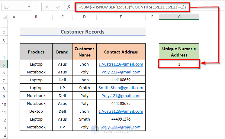
Formula Breakdown
ISNUMBER(E5:E13): For all the addresses that are numeric values, returns TRUE; FALSE otherwise.
COUNTIFS(E5:E13,E5:E13): For all addresses that show just once, returns TRUE;FALSE otherwise.
ISNUMBER(E5:E13)*COUNTIFS(E5:E13,E5:E13): multiplies the ISNUMBER formula and COUNTIFS formula. It returns 1 if criteria are met; 0 otherwise.
SUM(--(ISTEXT(E5:E13)*COUNTIFS(E5:E13,E5:E13)=1)): returns the unique number values.
Download Practice Workbook
Download the workbook and practice.
<< Go Back to Learn Excel
Get FREE Advanced Excel Exercises with Solutions!
