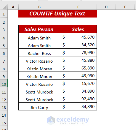
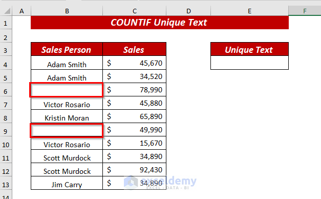
We’ll use a sample dataset of sales information. The dataset contains two columns: Sales Person and Sales. Let’s extract the unique values.
How to Use COUNTIF for Unique Text: 8 Ways
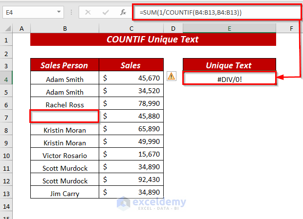
Method 1 – Using SUM and COUNTIF Functions to Count Unique Text
- In cell E4, use the following formula.
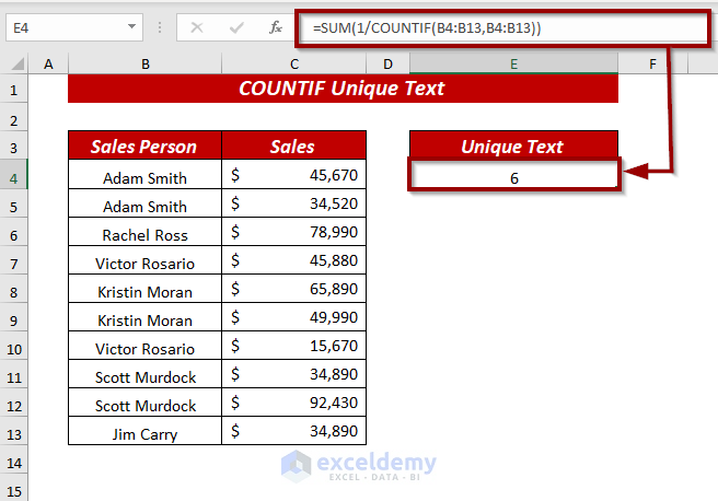
=SUM(1/COUNTIF(B4:B13,B4:B13))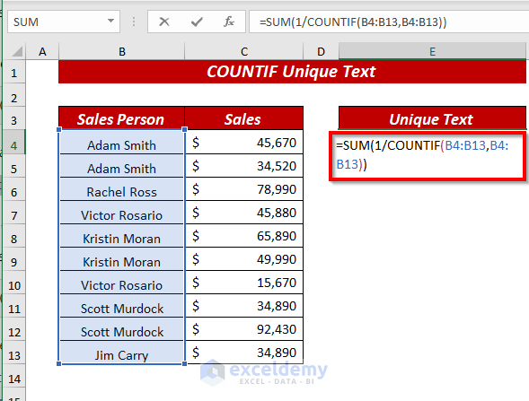
We used 1/COUNTIF(B4:B13,B4:B13) as number1. In the COUNTIF function, B4:B13 is the range, and B4:B13 as the criteria. We put 1 as a dividend to divide the return array (which is the divisor) of the COUNTIF function.
The SUM function will return the total of all numbers in the list.
Formula Breakdown
➦ COUNTIF(B4:B13,B4:B13) —> It will find out how many times each individual value appears in the specified range.
Output : {2;2;1;2;2;2;2;2;2;1}
➦ 1/COUNTIF(B4:B13,B4:B13 —> becomes
Output : {0.5;0.5;1;0.5;0.5;0.5;0.5;0.5;0.5;1}
➦ SUM(1/COUNTIF(B4:B13,B4:B13)) —> becomes
Output : 6
- Press Ctrl + Shift + Enter keys and you will get the count of Unique Text.
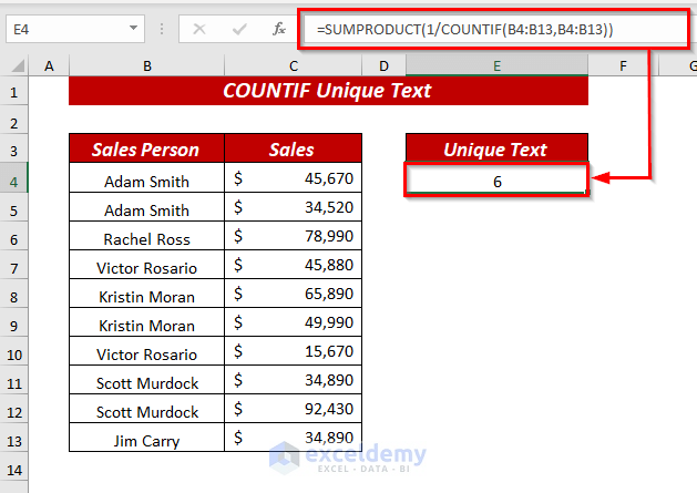
Method 2 – Using SUMPRODUCT and COUNTIF Functions to Get the Distinct Unique Text
- In cell E4, use the following formula.
=SUMPRODUCT(1/COUNTIF(B4:B13,B4:B13))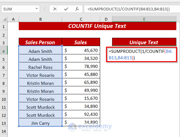
In the SUMPRODUCT function, we used 1/COUNTIF(B4:B13,B4:B13) as array1. In the COUNTIF function, we used the B4:B13 as range and B4:B13 as criteria. The 1 is a dividend to divide the return value of the COUNTIF function.
- Press the Enter key and you will get the Unique Text count.
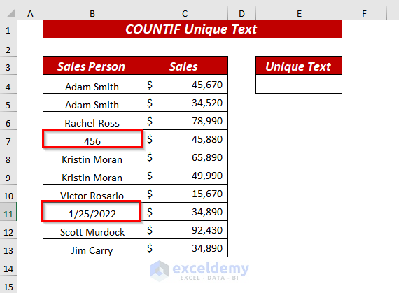
Method 3 – COUNT Only Unique Text Values Ignoring Numeric and Date Values
We slightly changed my dataset by inserting a numeric value and a date value in the Sales Person column.
- In cell E4, use the following formula.
=SUM(IF(ISTEXT(B4:B13),1/COUNTIF(B4:B13, B4:B13),""))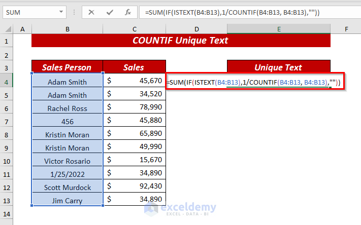
In the SUM function, we used IF(ISTEXT(B4:B13),1/COUNTIF(B4:B13, B4:B13),””) as number1. In the IF function, we used ISTEXT(B4:B13) as the logical_test, 1/COUNTIF(B4:B13, B4:B13) as value_if_true, and “” (Blank) for value_if_false. In the ISTEXT function, I selected the range B4:B13 as a value.
If the cell contains text, ISTEXT will return TRUE, then the function will provide a value. Otherwise, it returns a blank and goes to the next cell.
In the COUNTIF function, we used B4:B13 as range and B4:B13 as criteria. We used 1 as a dividend to divide the return array of the COUNTIF function. The SUM function will return the total of all numbers in the list.
Formula Breakdown
➦ COUNTIF(B4:B13,B4:B13) —> It will find out how many times each individual value appears in the specified range.
Output : {2;2;1;1;2;2;1;1;1;1}
➦ 1/COUNTIF(B4:B13,B4:B13 —> becomes
Output : {0.5;0.5;1;1;0.5;0.5;1;1;1;1}
➦ ISTEXT(B4:B13) —> becomes
Output : {TRUE;TRUE;TRUE;FALSE;TRUE;TRUE;TRUE;FALSE;TRUE;TRUE}
➦ IF(ISTEXT(B4:B13),1/COUNTIF(B4:B13, B4:B13),””) —> becomes
Output : {0.5;0.5;1; ;0.5; 0.5 ;1; ;1;1}
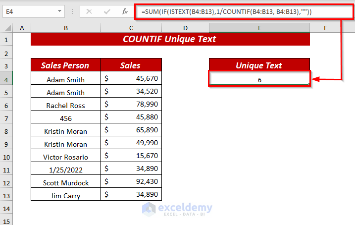
➦ SUM(IF(ISTEXT(B4:B13),1/COUNTIF(B4:B13, B4:B13),””)) —> becomes
Output : 6
- Press Enter.
Method 4 – Count Unique Text Values Ignoring Empty Cells
Let’s remove some values from the dataset.
- In cell E4, use the following formula.
=SUM(IF(B4:B13<>"",1/COUNTIF(B4:B13, B4:B13), 0))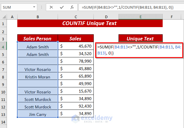
In the SUM function, we used IF(B4:B13<>””,1/COUNTIF(B4:B13, B4:B13), 0) as number1.
In the IF function, we used B4:B13<>”” as logical_test, 1/COUNTIF(B4:B13, B4:B13 as value_if_true, and 0 as value_if_false. If any cell is empty in the selected range, then IF will return 0 instead of calculating the result for that cell.
The 1 is used to divide the return array (which is the divisor) of the COUNTIF function. The SUM function will return the total of all numbers in the list.
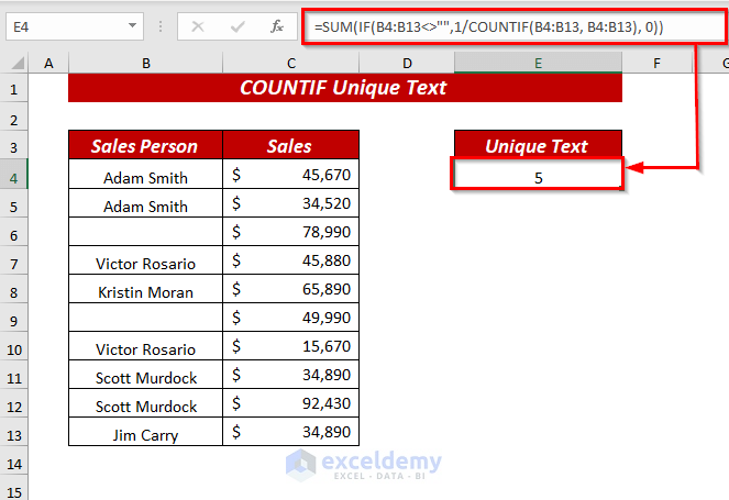
- Press the Enter key and you will get the Unique Text count while ignoring empty cells.
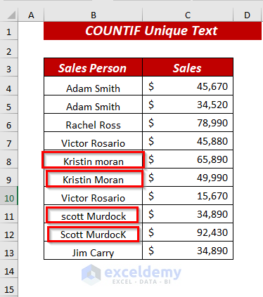
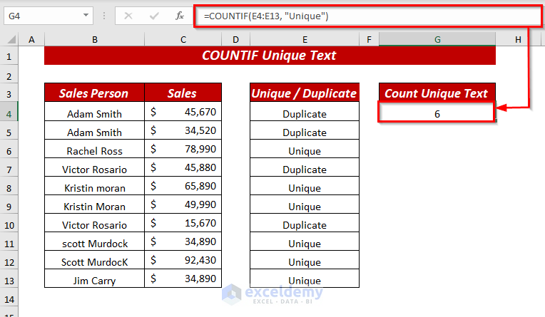
Method 5 – Get Case-Sensitive Unique Text Using COUNTIF
We slightly changed some values in the dataset to have various spellings in different cases.
- In cell E4, use the following formula.
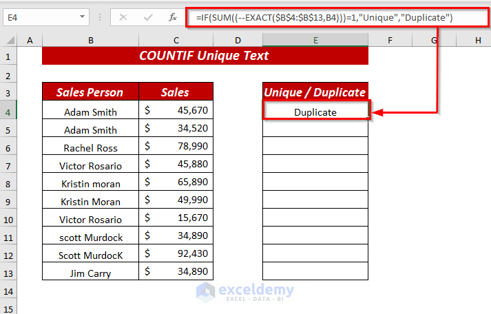
=IF(SUM((--EXACT($B$4:$B$13,B4)))=1,"Unique","Duplicate")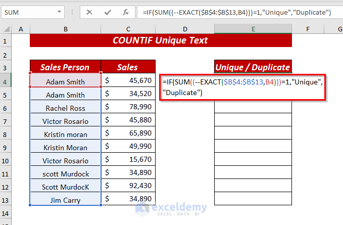
In the IF function, we used SUM((–EXACT($B$4:$B$13,B4)))=1 as logical_test , Unique as value_if_true and Duplicate as value_if_false.
In the SUM function, we used (–EXACT($B$4:$B$13,B4)) as number1. In the EXACT function, we selected the range $B$4:$B$13 as text1 and B4 as text2. The EXACT function will return a binary value 1 if text1 matches with text2, or 0 otherwise. (–EXACT($B$4:$B$13,B4))=1 will convert the binary result into a boolean TRUE or FALSE. Then the IF function will check the returned value of the EXACT function. If the value is TRUE, then it will return Unique. Otherwise, the result becomes Duplicate.
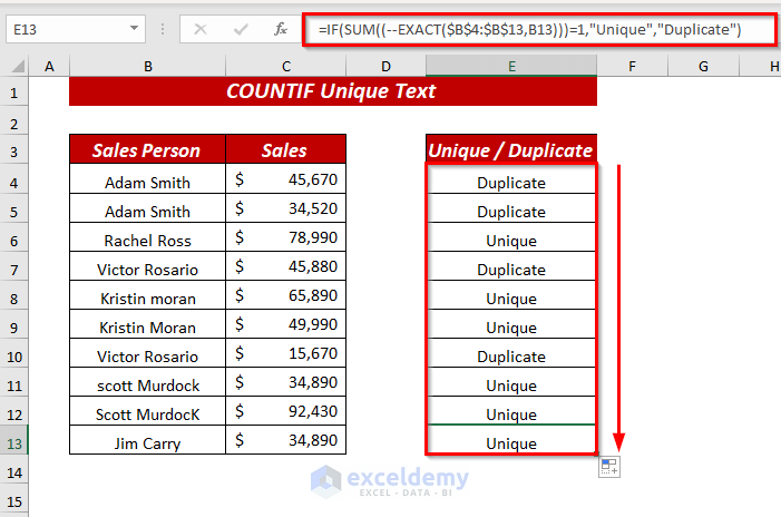
- Press the ENTER key and you will get the exact match result.
- Use the Fill Handle to AutoFill the formula for the rest of the cells.
- In cell G4, use the following formula.
=COUNTIF(E4:E13, "Unique")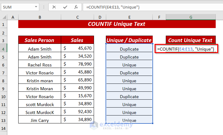
The function will count all the unique values from the selected range.
- Press the Enter key and you will get the Unique Text count.
Method 6 – Combining SUM and COUNTIF Functions to Count Unique Text (Only Occurred Once)
- In cell E4, insert the following formula.
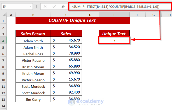
=SUM(IF(ISTEXT(B4:B13)*COUNTIF(B4:B13,B4:B13)=1,1,0))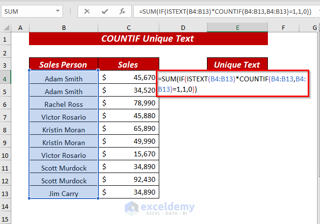
In the SUM function, we used IF(ISTEXT(B4:B13)*COUNTIF(B4:B13,B4:B13)=1,1,0) as number1.
In the IF function, we used ISTEXT(B4:B13)*COUNTIF(B4:B13,B4:B13)=1 as logical_test, 1 as value_if_true, and 0 as value_if_false.
In the ISTEXT function, we selected the range B4:B13 as the value. If the cell value is text, it will return TRUE. Otherwise, it returns FALSE.
In the COUNTIF function, we used B4:B13 as range and B4:B13 as criteria. ISTEXT(B4:B13)*COUNTIF(B4:B13,B4:B13)=1 will convert the result into boolean (TRUE or FALSE). Then, the IF function will check the logical_test_value. If the value is TRUE, it will return 1.
The SUM function will return the total of all numbers in the list.
- Press the ENTER key and you will get only the Unique Text that occurred only once.
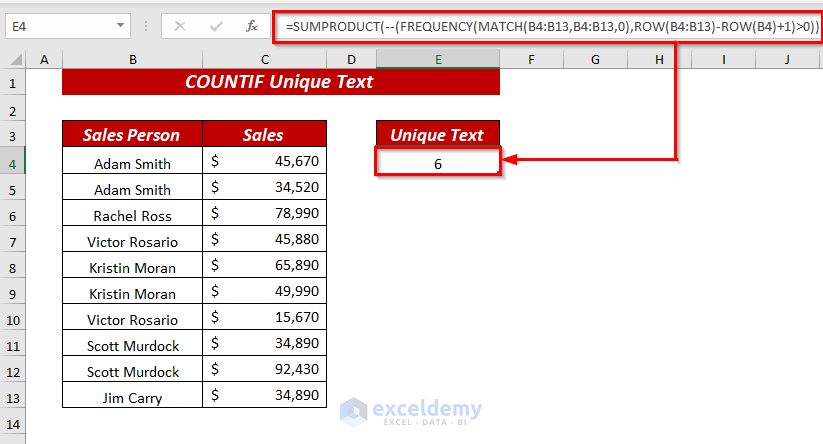
Method 7 – Using SUMPRODUCT and FREQUENCY Functions to Count Unique Text
- In cell E4, use the following formula.
=SUMPRODUCT(--(FREQUENCY(MATCH(B4:B13,B4:B13,0),ROW(B4:B13)-ROW(B4)+1)>0))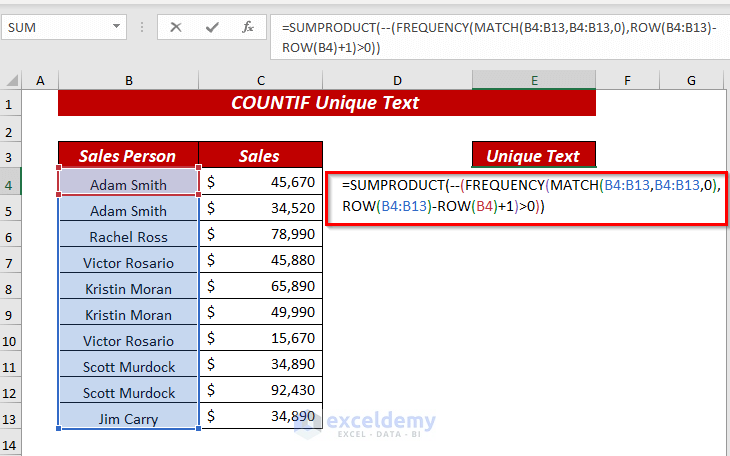
In the SUMPRODUCT function, we used –(FREQUENCY(MATCH(B4:B13,B4:B13,0),ROW(B4:B13)-ROW(B4)+1)>0) as array1.
For the FREQUENCY function, we used MATCH(B4:B13,B4:B13,0) as data_array and ROW(B4:B13)-ROW(B4)+1 as bins_array.
In the MATCH function, we selected the range B4:B13 as the lookup_value, B4:B13 as lookup_array, and 0 as match_type where 0 means exact match. This will return the position of the first match, so values that appear more than once in the data return the same position. This array will be fed into the FREQUENCY function as data_array.
In the ROW function, we used B4:B13 as a reference. ROW(B4:B13)-ROW(B4)+1 will return a sequential list of numbers for each value in the data and it is fed into the FREQUENCY function as bins_array.
The FREQUENCY function will return an array of numbers that indicate a count for each number in the data array which is organized by bins numbers for each value in the data.
The SUMPRODUCT function will check the values that are greater than 0 and will convert the result into TRUE or FALSE. We used a Double Negative (–) sign to convert the boolean result into a binary number.
- Press the Enter key to get the result.
Method 8 – Using SUM and FREQUENCY Functions to Count Unique Text Based on Criteria
We’ve put a separate cell as a criterion to filter the table by in the formula.
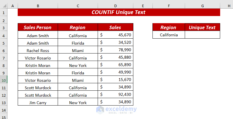
- In cell G4, use the following formula.
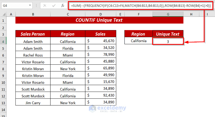
=SUM(--(FREQUENCY(IF(C4:C13=F4,MATCH(B4:B13,B4:B13,0)),ROW(B4:B13)-ROW(B4)+1)>0))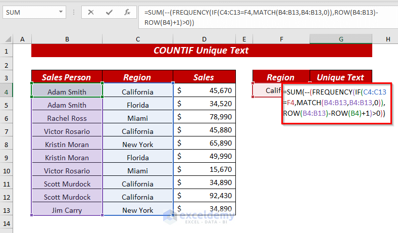
In the SUMPRODUCT function, we used –(FREQUENCY(IF(C4:C13=F4,MATCH(B4:B13,B4:B13,0)),ROW(B4:B13)-ROW(B4)+1)>0) as array1.
In the FREQUENCY function, we used IF(C4:C13=F4,MATCH(B4:B13,B4:B13,0)) as data_array and ROW(B4:B13)-ROW(B4)+1 as bins_array.
For the IF function, we used C4:C13=F4 as logical_test and MATCH(B4:B13,B4:B13,0) as value_if_true.
In the MATCH function, the range B4:B13 is a lookup_value, B4:B13 as lokkup_array, and 0 as match_type means exact match. It will return the position of the first match, so values that appear more than once in the data return the same position.
The IF function acts as a filter, and it will only allow the values from MATCH to pass through if the value in the cell in column C is equal to the F4 cell.
In the ROW function, we used B4:B13 as a reference. ROW(B4:B13)-ROW(B4)+1 will return a sequential list of numbers for each value in the data and it is fed into the FREQUENCY function as bins_array.
The FREQUENCY function will return an array of numbers that indicate a count for each number in the data array which is organized by bins numbers for each value in the data.
The SUM function will check the values that are greater than 0 and will convert the result into TRUE or FALSE. We used the Double Negative (–) sign to convert the boolean result into a binary number (1 or 0).
- Press the Ctrl + Shift + Enter keys to get the result.
Things to Remember
While using the array formula remember to press Ctrl + Shift + Enter key. Excel 365 users can use Enter only.
You will get the #DIV/0! error if you have empty cells unless you use a method to ignore them.
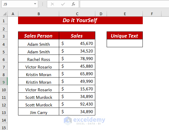
Practice Section
We’ve provided a practice sheet in the workbook so you can experiment.
Download the Practice Workbook
<< Go Back to Learn Excel
Get FREE Advanced Excel Exercises with Solutions!
