How to Count Unique Names in Excel (6 Simple Methods)

In this article, we will demonstrate some methods to count unique names in Excel. Excel doesn’t have a built-in function to count unique values or text, but there are a variety of techniques and approaches by which we can count these distinct values.

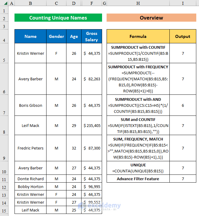
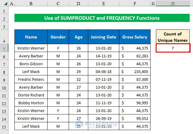
In the following image is an overview of the methods we’ll use.

Method 1 – Using the SUMPRODUCT Function to Count Unique Names in Excel

The simplest and easiest way to count unique names in Excel is by using the SUMPRODUCT function. Using this function, we can count unique values in two ways.

1.1 – Combining SUMPRODUCT with COUNTIF

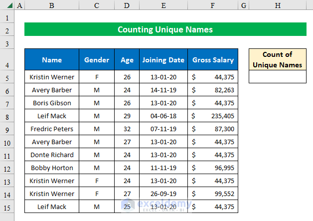
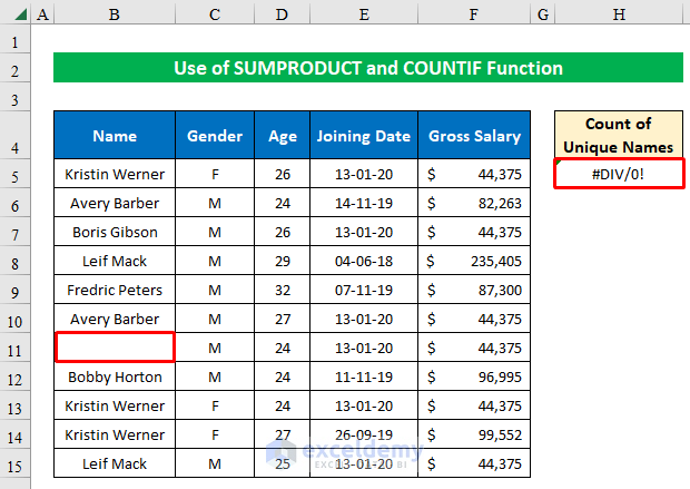
In the dataset below we have some Employee Names and their Gross Salary. Some Employee Names appear more than once. We’ll count the number of unique Employee Names in cell H5 under the heading “Count of Unique Names”.

Steps:

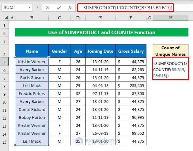
In cell H5, apply the SUMPRODUCT function with the COUNTIF function.

The generic formula is:

=SUMPRODUCT(1/COUNTIF(range,criteria))

Insert the values into the function and the final form of the formula is:

=SUMPRODUCT(1/COUNTIF(B5:B15,B5:B15))

Where,

The range and Criteria are B5:B15.
The COUNTIF function looks into the data range and counts the number of times each name appears.
- Output: {3;2;1;2;1;2;1;1;3;3;2}
The result of the COUNTIF function is used as the divisor, with 1 as the numerator. As a result, numbers that appeared only once in the array become 1 and numbers with multiple instances provide fractions as results.
Finally, the SUMPRODUCT function will count the 1‘s and return the result.

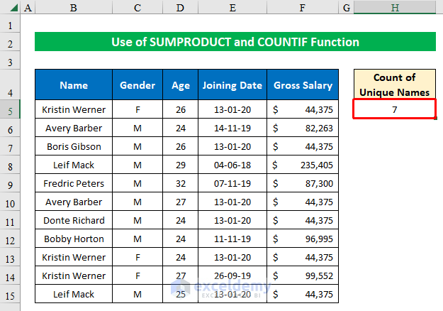
Press ENTER to return the unique values.

There is a flaw in this function. If there is a Blank Cell in the data set, then the formula will fail because the COUNTIF function generates “0” for each blank cell, and 1 divided by 0 returns a divide by zero error (#DIV/0!).

To overcome this situation let’s modify the formula a bit:

=SUMPRODUCT(((B5:B15<>"")/COUNTIF(B5:B15,B5:B15&"")))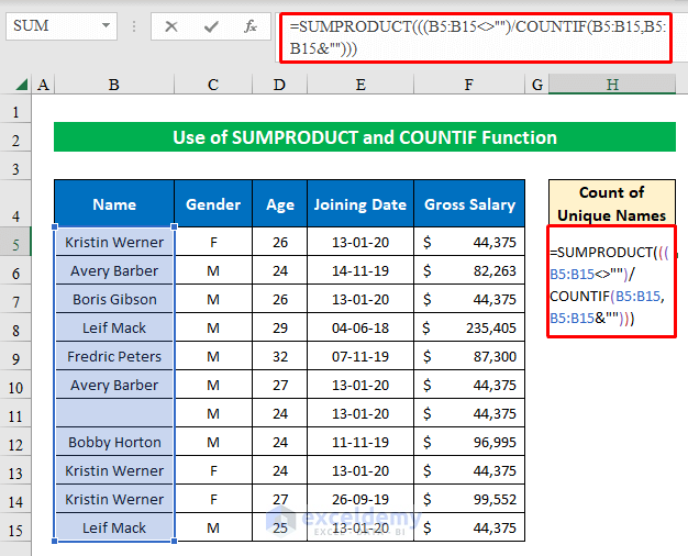

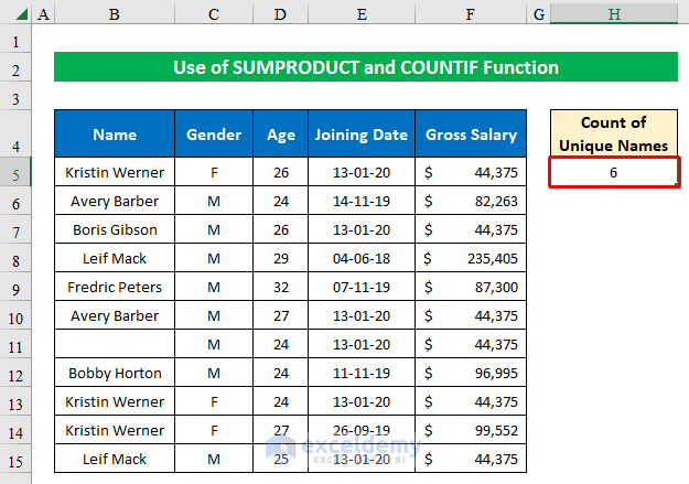
Now if there is any blank cell in the dataset, the formula will ignore it.

Press ENTER to get the result.

1.2 – Combining SUMPRODUCT with FREQUENCY

We will use the same data range here that we used in the previous example.

Steps:

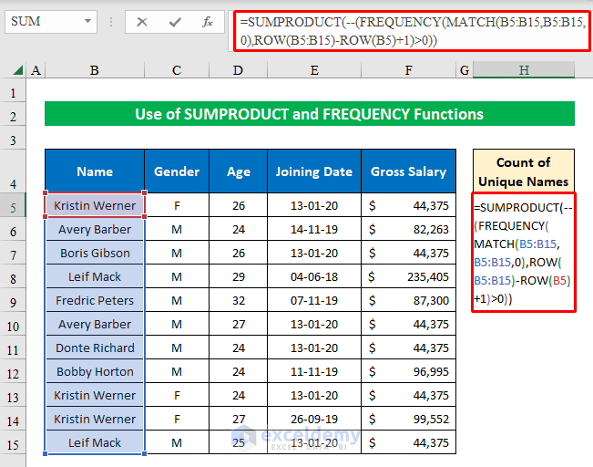
Apply the SUMPRODUCT function combined with the FREQUENCY function to get the unique names.

The generic formula is:

=SUMPRODUCT(--(FREQUENCY(MATCH(Lookup_value,Lookup_array,[match_type])),ROW(reference)-ROW(reference.firstcell)+1),1))

Insert the values to get the final form:

=SUMPRODUCT(--(FREQUENCY(MATCH(B5:B15,B5:B15,0),ROW(B5:B15)-ROW(B5)+1)>0))

Where,

The MATCH function is used to get the position of each name that appears in the data. Here in the MATCH function the lookup_value, lookup_array and [match type] are B5:B15,B5:B15,0.
The bins_array argument is constructed from this part of the formula: (ROW(B5:B15)-ROW(B5)+1)
The FREQUENCY function returns an array of numbers which represent a count of each number in the array of data, organized by bin. A key feature in the operation of the FREQUENCY formula is that when a number has already been counted, FREQUENCY will return zero.
Now we check for values that are greater than zero (>0), which converts the numbers to TRUE or FALSE, then we use a double-negative (– –) to convert the TRUE and FALSE values to 1s and 0s.
Finally, the SUMPRODUCT function simply adds the numbers up and returns the total.

Since this is an Array Formula, press “CTRL+SHIFT+ENTER” to apply the formula.

We have our final count.

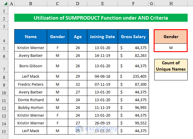
Method 2 – Using SUMPRODUCT Under AND Logic to Count Unique Names with Criteria

We can also utilize the SUMPRODUCT function under AND logic to count unique names with criteria.

Suppose we have a criterion given in cell H5 which is “M”. Let’s count the unique names that match the criteria.

Steps:

Choose a cell (H8) and enter the formula below:

=SUMPRODUCT((C5:C15=H5)*(1/COUNTIF(B5:B15,B5:B15)))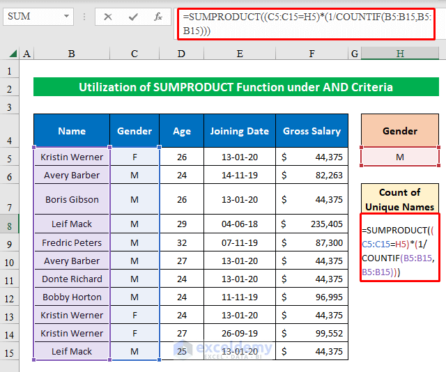

Press ENTER to return the count of the unique names.

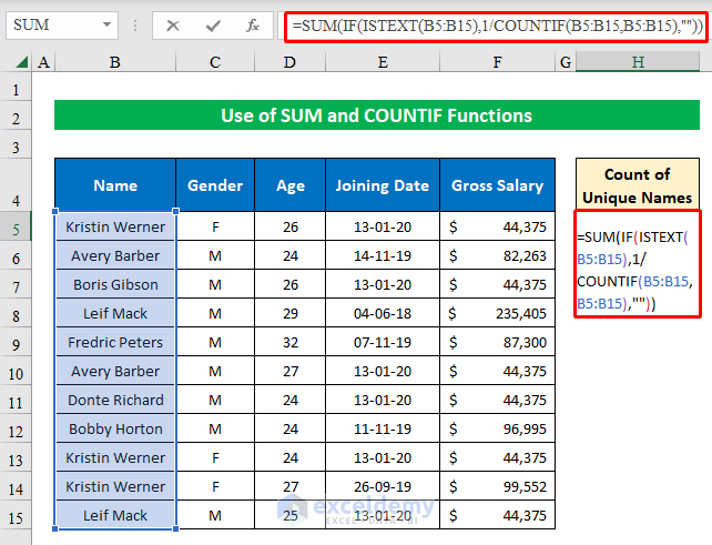
Method 3 – Using the SUM Formula with the COUNTIF Formula to Count Unique Names in Excel

Here’s a different approach.

Steps:

Here, we will use the SUM with COUNTIF formula to get the required count.

The generic formula is:

=SUM(IF(ISTEXT(Value),1/COUNTIF(range, criteria), ""))

Insert the values to get the final form of the formula:

=SUM(IF(ISTEXT(B5:B15),1/COUNTIF(B5:B15,B5:B15),""))

Where,

The ISTEXT function returns TRUE for all the values that are text and false for other values.
The Range and Criteria are B5:B15
If the value is a text value, the COUNTIF function looks into the data range and counts the number of times each name appears in the data range.
- Output: {3;2;1;2;1;2;1;1;3;3;2}
The SUM function computes the sum of all the values and returns the result.

Since this is an Array Formula, press “CTRL+SHIFT+ENTER” to apply the formula.

We have our final count.

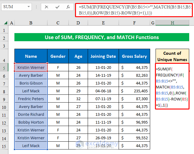
Method 4 – Combining the SUM, FREQUENCY and MATCH Functions to Count Unique Names

In some situations, we can also combine the SUM, FREQUENCY, and MATCH functions to count unique names.

The generic formula is:

=SUM(IF(FREQUENCY(IF(logical test<>"", MATCH(Lookup_value,Lookup_array,[match type])),ROW(reference)-ROW(reference.firstcell)+1),1))

Steps:

The final formula after value insertion is:

=SUM(IF(FREQUENCY(IF(B5:B15<>"",MATCH(B5:B15,B5:B15,0)),ROW(B5:B15)-ROW(B5)+1),1))

Where,

In the MATCH function the lookup_value, lookup_array and [match type] are B5:B15,B5:B15,0.
After the MATCH function there is an IF, which is needed because MATCH will return an #N/A error for empty cells. We exclude the empty cells in the IF function with B5:B15<>””.
The bins_array argument is constructed from this part of the formula: (ROW(B5:B15)-ROW(B5)+1)
This resulting array is fed to the FREQUENCY function which returns an array of numbers that represent a count for each number in the array of data.
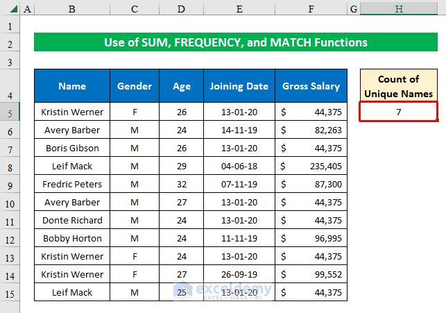
Finally, the outer IF function indicates each unique value as 1 and each duplicate value as 0.

Press “CTRL+SHIFT+ENTER” to apply the array formula.

Method 5 – Using the UNIQUE Function to Count Unique Names in Excel

The UNIQUE function is only available in the Excel 365 version.

Step 1:

Apply the UNIQUE function. The generic formula is:

=COUNTA(UNIQUE(range))

After inputting the values, the final form is:

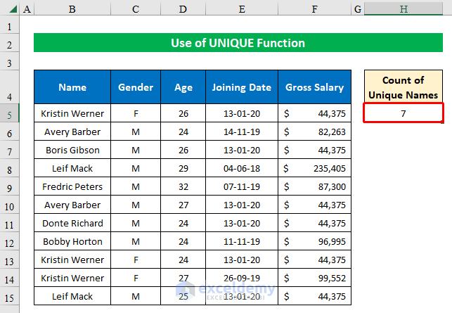
=COUNTA(UNIQUE(B5:B15))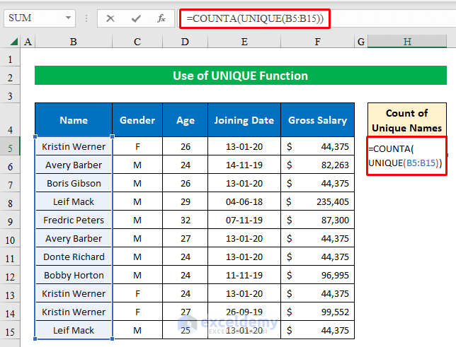

Press ENTER to get the result.

Step 2:

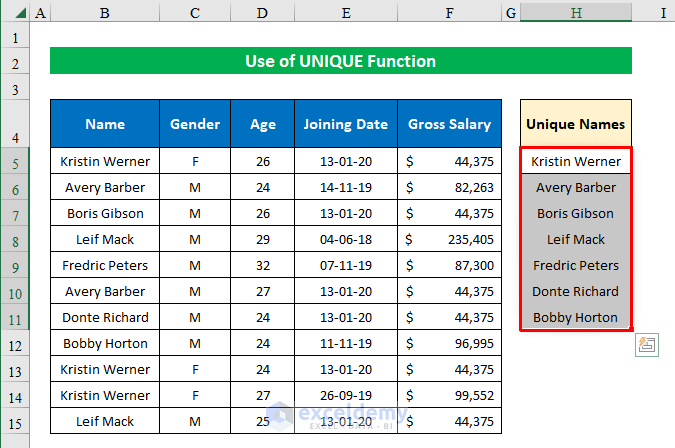
We can also get the list of unique names by using this UNIQUE formula:

=UNIQUE(B5:B15)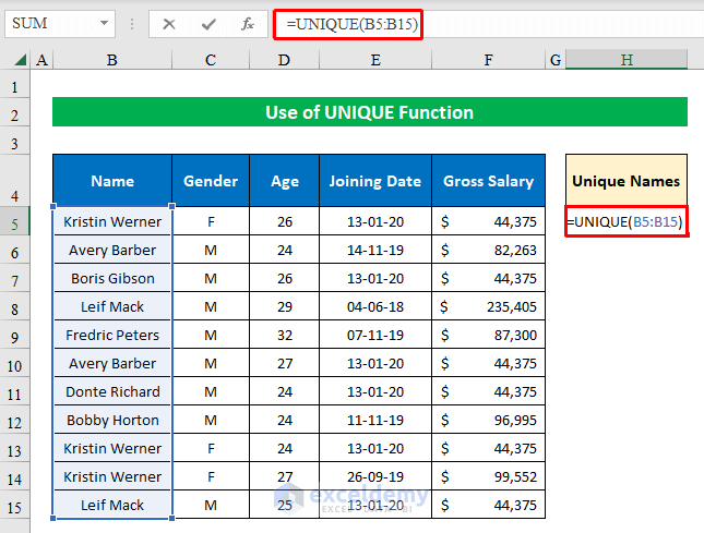

Press ENTER to return the result.

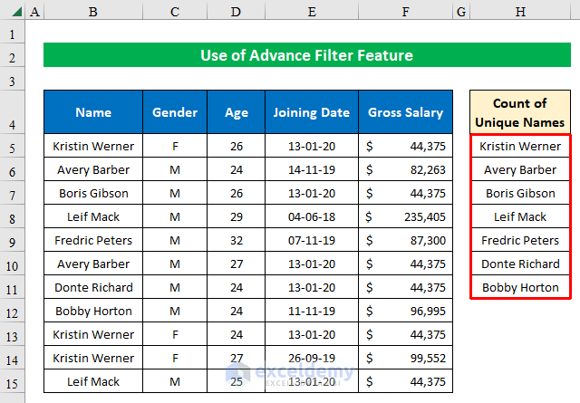
Method 6 – Applying the Advanced Filter to Count Unique Names in Excel

We can also use the Advanced Filter option to count unique names.

Steps:

Go to the Data tab.
In the Sort & Filter group, click on Advanced.

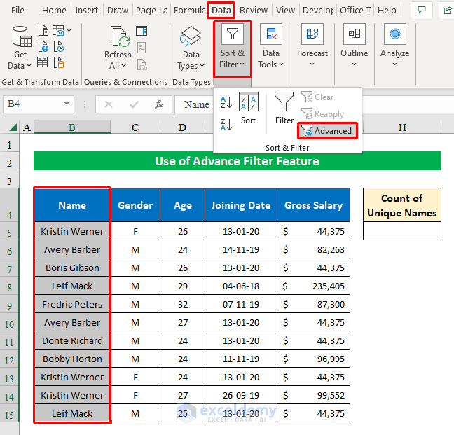
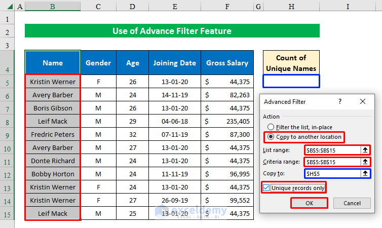
The Advanced Filter window appears.

Choose Copy to Another Location and check Use Unique Records Only.
Select the data source for the List Range ($B$5:$B$15), Criteria Range ($B$5:$B$15), and Copy to ($H$5).
Click OK to continue.

Our list of unique names is complete.

To count the unique names, use this formula and press ENTER:

=ROWS(H5:H11)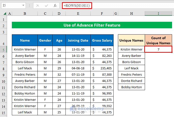

Quick Notes

➤ If there is a blank cell in the dataset when you are using the SUMPRODUCT with COUNTIF formula, the result will show a divide by zero error (#DIV/0!)

➤ For the Array Formula, press “CTRL+SHIFT+ENTER” simultaneously to get the result.

➤ The UNIQUE function is only available in Excel 365. Users of older versions of Excel won’t be able to use the function.

Download Practice Workbook

Count Unique Names.xlsx

<< Go Back to Learn Excel

Get FREE Advanced Excel Exercises with Solutions!