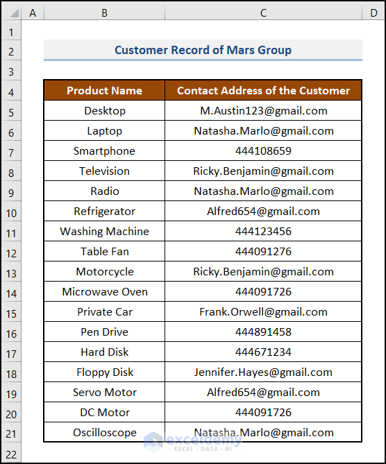
We’re going to use a Customer Record of Mars Group. This sample dataset includes some Product Names and Contact Addresses of the Customers who bought the products from this company. We’ll count the total number of unique text values and numerical values from the contact addresses.
Method 1 – Using COUNTIFS for Counting Unique Text Values in Excel
Steps:
- Select cell B24 and enter the following formula:
=SUM(--(ISTEXT(C5:C21)*COUNTIFS(C5:C21,C5:C21)=1))Formula Breakdown
- ISTEXT(C5:C21) returns TRUE for all the addresses that are text values and returns FALSE for all the addresses that are not text values.
- COUNTIFS(C4:C20,C4:C20)=1 returns TRUE for all the addresses that appear only once, and FALSE for the addresses that appear more than once.
- –(ISTEXT(C4:C20)*COUNTIFS(C4:C20, C4:C20)=1) multiplies the two conditions and returns 1 if both the conditions are met, otherwise returns 0.
- The SUM function adds all the values and returns the number of unique text values.
- Hit the Enter key.

Note: This is an Array Formula. Press Ctrl + Shift + Enter if you’re not using Office 365.
You can perform the same operation using the COUNTIF function in Excel. As you can see, there are three distinct text addresses.
Read more: How to Use COUNTIF for Unique Text
Method 2 – Counting Unique Numerical Values with the COUNTIFS Function
Steps:
- Go to cell B24 and insert the formula below:
=SUM(--(ISNUMBER(C5:C21)*COUNTIFS(C5:C21,C5:C21)=1))Formula Breakdown
- ISNUMBER(C5:C21) returns TRUE for all the addresses that are numerical values and returns FALSE for all the addresses that are not numerical values.
- COUNTIFS(C5:C21,C5:C21)=1 returns TRUE for all the addresses that appear only once, and FALSE for the addresses that appear more than once.
- –(ISNUMBER(C4:C20)*COUNTIFS(C4:C20, C4:C20)=1) multiplies the two conditions and returns 1 if both the conditions are met, otherwise returns 0.
- The SUM function adds all the values and returns the number of unique numerical values.
- Hit Enter.

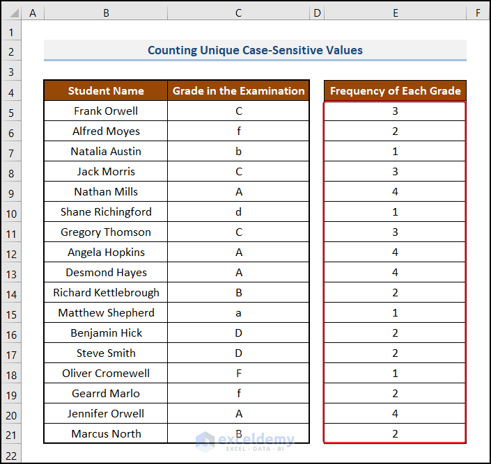
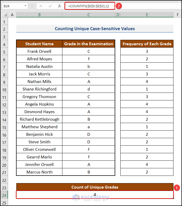
Method 3 – Counting Unique Case-Sensitive Values Using COUNTIFS in Excel
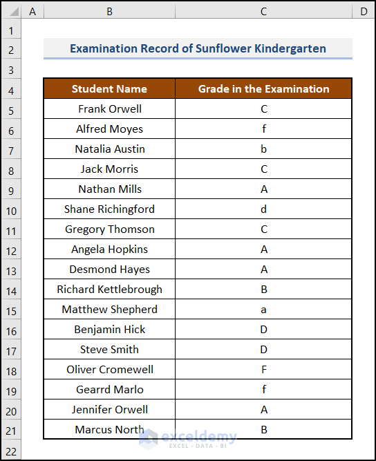
We have an Examination Record of Sunflower Kindergarten. It contains the grades of some students. We want to count the total number of unique grades considering case-sensitive matches.
Steps:
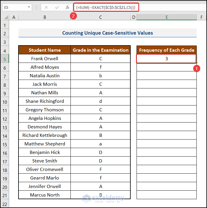
- Construct a new column with the heading Frequency to Each Grade and enter the following formula in the first cell (cell E5) of this column:
=SUM(--EXACT($C$5:$C$21,C5))- Hit Enter.
- Bring the cursor to the bottom-right corner of cell E5 and it’ll look like a plus (+) sign. This is the Fill Handle tool.
- Double-click on it.
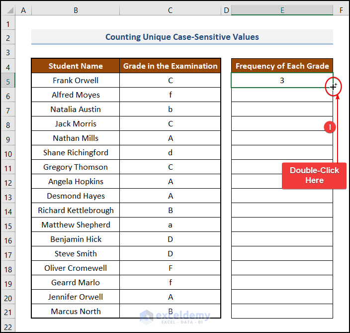
- This copies the formula to the lower cells, and the remaining cells get outputs.
- Create an output range in cells in the B23:E24 range.
- Go to cell B24 and use the following formula.
=COUNTIFS($E$5:$E$21,1)This is also an array formula.
- Hit Enter. You’ll get the case-insensitive count of unique grades.
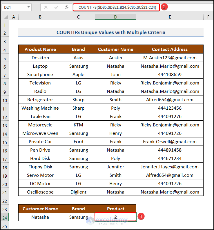
Method 4 – Inserting COUNTIFS to Count Unique Values with Multiple Criteria
Here the criteria are Customer Name and Brand, and we will count the products if they fulfill those criteria. We will primarily count only those products whose customer names and brands are the same.

Steps:
- Select the cell where you want the result. We selected cell D24.
- Insert the following formula:
=COUNTIFS($D$5:$D$21,B24,$C$5:$C$21,C24)Here, the range of cells D5:D21 indicates the Customer Name, and the criteria for this range is B24 which is Natasha. Also, the range of cells C5:C21 indicates the Brand, and the criteria for this range is C24 which is Samsung.
- Press Enter.
Limitations of the COUNTIFS Function to Count Unique Values in Excel
The formulas count the values that appear only once, but don’t count the total number of actual unique values present there, considering all the values. For example, if the range of values contains {A, A, A, B, B, C, D, E}, it will count only C, D, E, and return 3. But sometimes someone may need to count A, B, C, D, and E and return 5.
To solve these types of problems, Excel provides a function called the UNIQUE function in Office 365 only.
Alternative Way – Using the UNIQUE and ROWS Functions to Count Unique Values in Excel
- To count the unique number of contact addresses considering all the addresses, you can use this formula in cell B24.
=COUNTA(UNIQUE(C5:C21))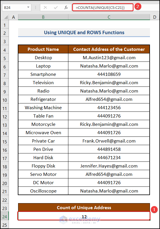
There are a total of 12 unique addresses (text and number), considering all the addresses at least once.
- To find the unique text addresses only, you can use this formula:
=ROWS(UNIQUE(IF(ISTEXT(C5:C21),C5:C21)))-1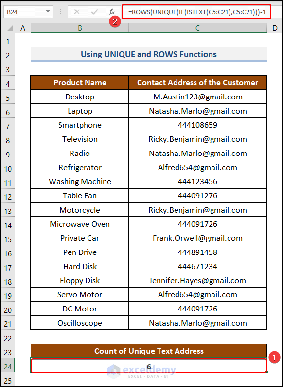
- To find the unique numerical addresses only, you can use the following formula in the same cell:
=ROWS(UNIQUE(IF(ISNUMBER(C5:C21),C5:C21)))-1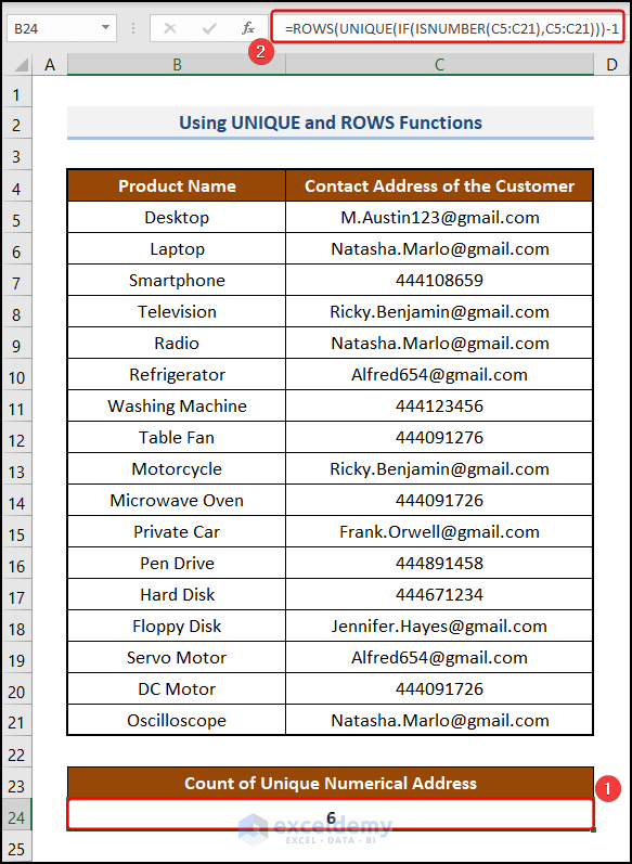
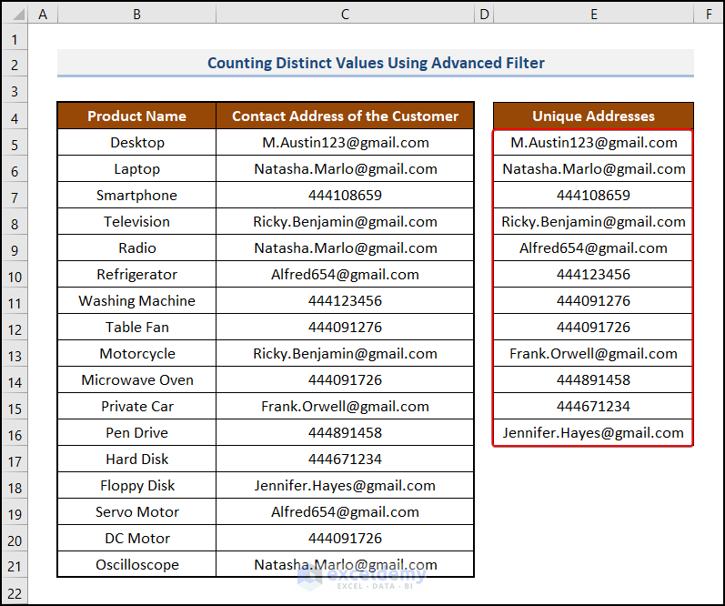
How to Count Distinct Values in Excel
Steps:
- Select cells in the C4:C21 range.
- Navigate to the Data tab.
- In the Sort & Filter group of commands, select the Advanced filtering option.
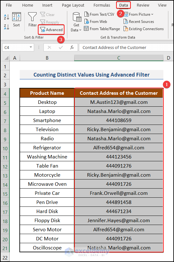
The Advanced Filter dialog box appears.
- In the Action area, select Copy to another location.
- Put C5:C21 in both the List range and Criteria range boxes.
- Make sure to check the box of Unique records only.
- Click OK.
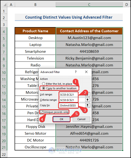
- This will create a new range of cells in the E5:E16 range.
- Go to cell E19 and paste the following formula.
=ROWS(E5:E16)- Press Enter.
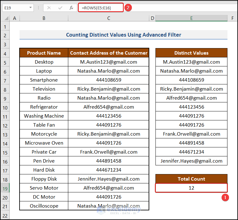
There are a total of 12 distinct address values in Column C.
Practice Section
We have provided a Practice section like the one below on each sheet on the right side so you can test these methods.

Download the Practice Workbook
<< Go Back to Unique Values | Learn Excel
Get FREE Advanced Excel Exercises with Solutions!

Great post! I really appreciate the step-by-step examples for using COUNTIFS with unique values. The tips you shared are super helpful for managing my data analysis tasks. Looking forward to trying out the methods you discussed!
Hello,
You are most welcome. Thanks for your feedback. Glad to hear that our articles step-by-step examples are helpful to manage data analysis. Keep exploring Excel with ExcelDemy!
Regards
ExcelDemy
Hi,
Is it possible to enter a formula which will add up the A’s in these cells please? I would expect the answer to be 11.
Thanks
Hello Erin,
Yes, you can use a formula to count how many times “A” appears in a range of cells. If the values are stored in a range like A1:A20, and each cell may contain multiple letters (e.g., “AB”, “AAB”), you can use this array formula (press Ctrl+Shift+Enter if you’re using an older version of Excel):
=SUM(LEN(A1:A20)-LEN(SUBSTITUTE(A1:A20,”A”,””)))
This formula calculates how many times “A” appears across the range. It should return 11 if there are exactly 11 “A”s in total.
Regards
ExcelDemy