Step 1 – Define Names for the Dropdown List
- Create dropdown boxes for 3 different items: Month, Year, and Shift.
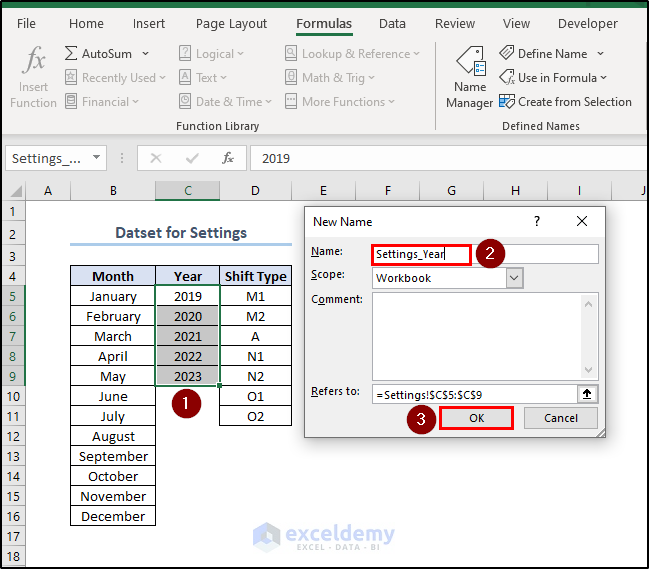
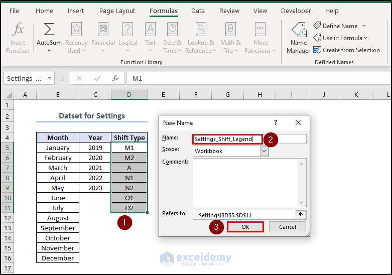
Let’s say we have five shifts from morning to night. M1, M2 represent morning shifts. A is for afternoon, and N1, N2 are for night shifts. There are also two off days defined by O1 and O2. Each employee has to work one shift each day, except for off days. Let’s define the names for the months with the help of Name Manager.
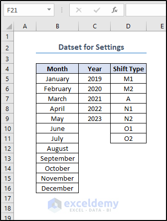
- Copy the range B5:B16.
- Select Define Name from the Formulas tab.
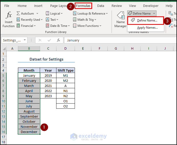
- A window will open where you have to define a name for range B5:B16. We named it Settings_Month.
- Press OK.
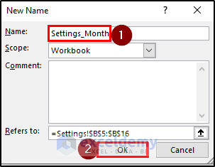
- Similarly, define the name for the Year. We named it Settings_Year.
- Define the Shift Type elements in the same procedure. We named it Settings_Shift_Legend.
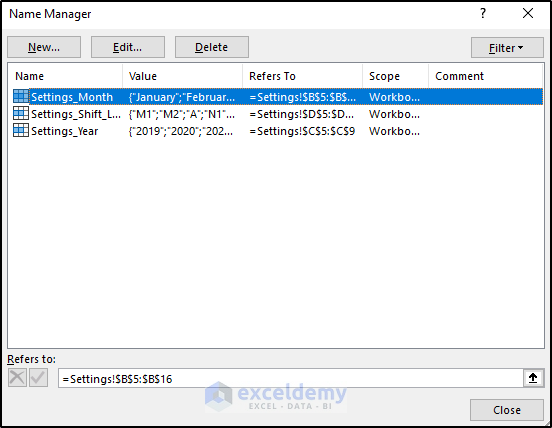
You can see all the names that have been defined by clicking the Name Manager option.

- If we click the Name Manager option, a window like this will open where you can see all the defined names.
Step 2 – Create Dropdown Lists with Data Validation
This is the outline of our Shift Roster. We will insert the Month and Year names in the dropdown boxes. Also, we need a dropdown box of Shift legends in each cell of the First Shift column. To create drop-down list, we’re going to use the Data Validation tool of Excel.
This Shift Roster can technically start anywhere in the month (e.g. 15 January – 14 February). You can set Month Start. This will automatically update the Start Date and End Date. We can set the First Shift. And the Roster will automatically update.
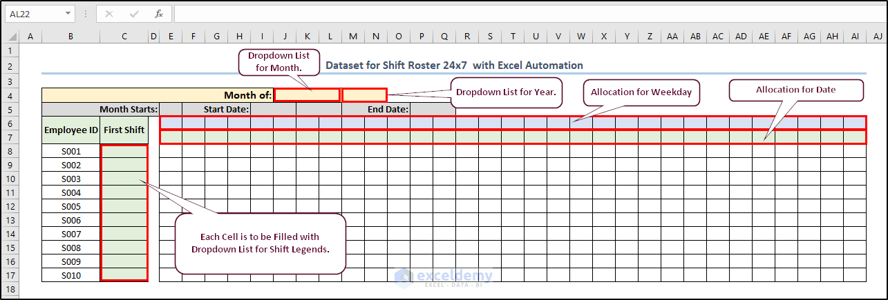
We have to create two dropdown boxes to specify which month of the year we are working with.
- Select the merged cell J4.
- Select Data Validation from the Data tab.
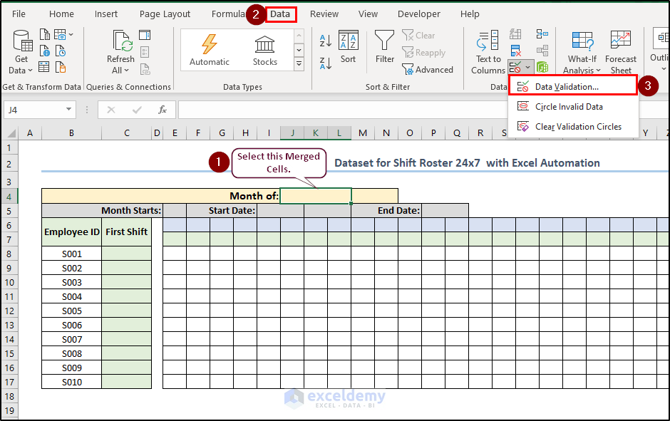
- A Data Validation will open to import the data source.
- Select List from the Allow dropdown box.
- Click on the Source box and press F3.
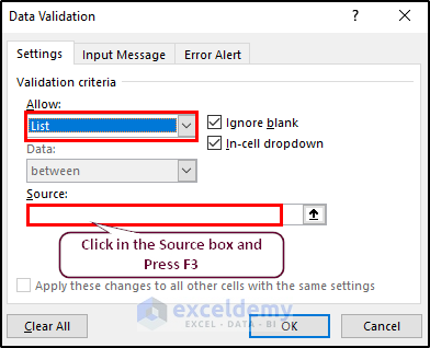
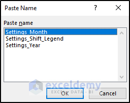
- A window named Paste Name will appear. You can see all the defined range names.
- Select Settings_Month and press OK.
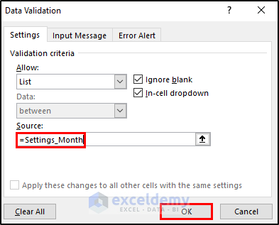
- We can see Settings_Month in the Source box of the Data Validation window.
- Now press OK.
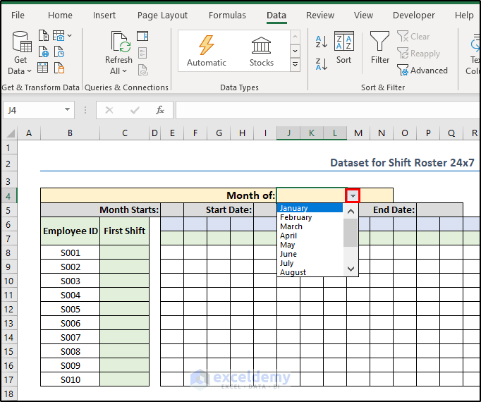
- Select the merged cell J4.
- You will see a dropdown arrow on the right side of the merged cell. You can select any month from there.
- Similarly, create a dropdown box in the merged cell M4 for Year.
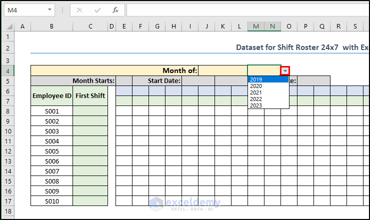
Now, we have to create dropdown boxes for each cell in the First Shift column.
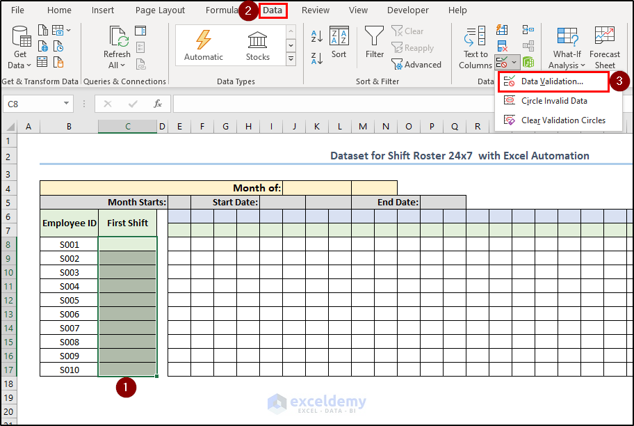
- Select all the cells from C8:C17.
- Import the defined name Settings_Shift_Legend through Data Validation as shown earlier.
Step 3 – Insert Formula for Relevant Fields
Let’s say we want to start at the beginning of the month:
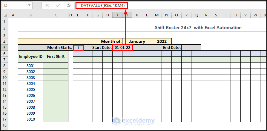
- Write 1 in the Month Start.
- Write the following formula in the Start Date box and press Enter.
= DATEVALUE(E5&J4&M4)This formula takes values from three cells and gives values in date.
- The start date will fill in. You might have to change the format to a date.
- Copy the following formula to the End Date box and press Enter.
=EOMONTH(I5,0) + E5 -1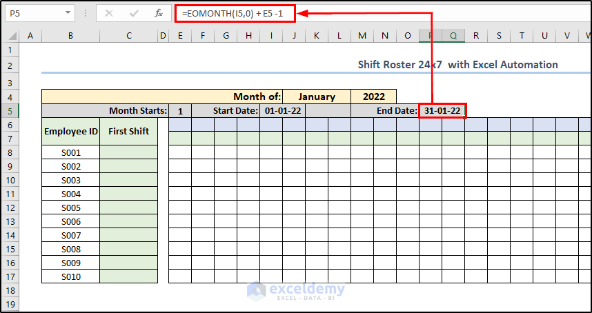
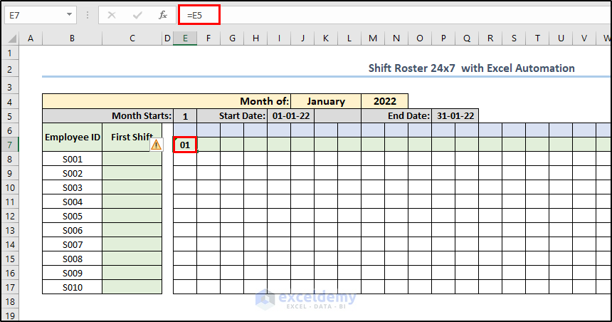
- Write =E5 in the E7 cell and press Enter. You will get “01” as the starting date.
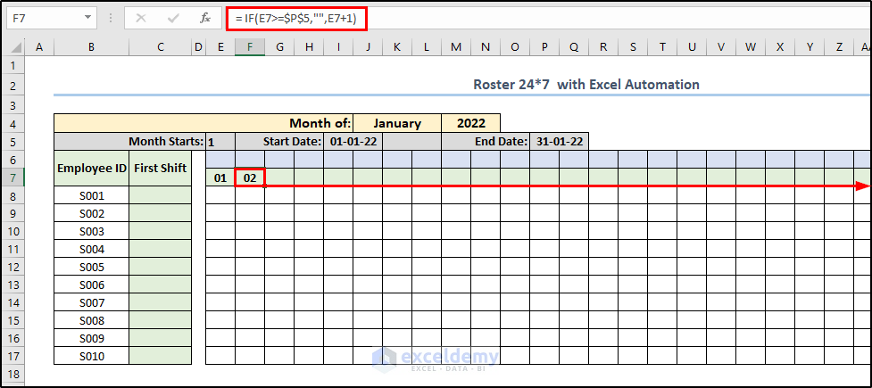
- Write the following formula in F7 and press Enter.
= IF(E7>=$P$5,"",E7+1)This formula gives sequential dates up to the End Date.
- Then hold and drag the F7 cell rightward to get all the dates.
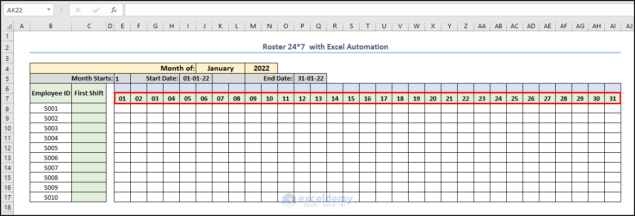
- By doing so, we have dates for the whole month.
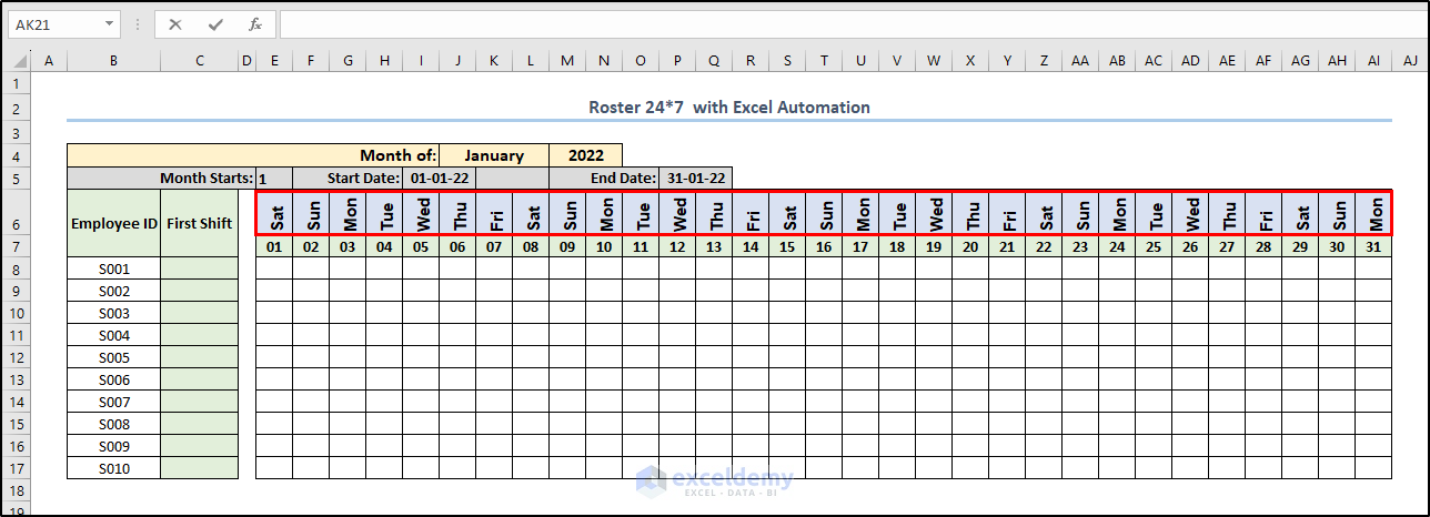
- Write the following formula in E6 and press Enter.
=TEXT(E7, "ddd")
This formula converts the dates into weekdays.
- Hold and drag the E6 cell rightward to get all weekdays.
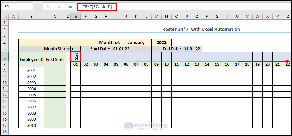
- Thereby, we get all weekdays. Modify the cell formatting so the text is rotated (Home > Orientation > Rotate Text Up).
Step 4 – Find Shift Roster for All Employees
- Select a First Shift.
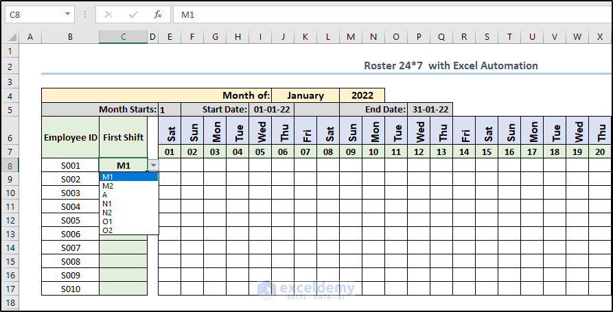
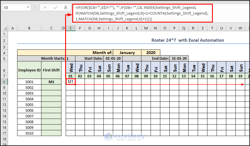
- Write the following formula in E8 and press Enter.
=IF(OR($C8="",E$7=""), "",IF(D8= "",C8, INDEX(Settings_Shift_Legend,IF(MATCH(D8,Settings_Shift_Legend,0)+1>COUNTA(Settings_Shift_Legend),1,MATCH(D8,Settings_Shift_Legend,0)+1))))This formula checks the First Shift cell($C8) and the upper date cell(E$7) if they both are blank. When both of them are blank, the formula returns an empty string.
If not, it checks if the previous shift cell(D8) is empty. If D8 is not empty it finds the value of D8 in the “Setting_Shift_Legend” range and returns the next shift legend.
It returns the value of C8 if D8 is empty.
In short, this formula gives sequential Shifts for each employee.
This will give you M1.
- Hold and drag the first result cell to the right to get Shift Roster for the first employee.
- Then hold and drag the entire selected range downwards to copy the formula from E8 to AI17.
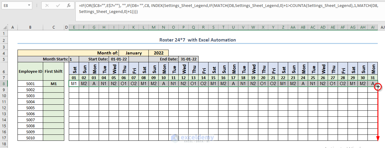
- For the second employee’s First Shift, select M2.
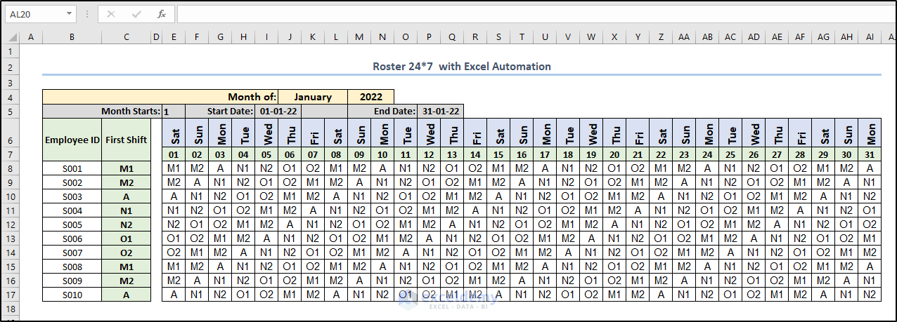
And the second row will be filled with Shift legends indicating the employee’s shift on each date.
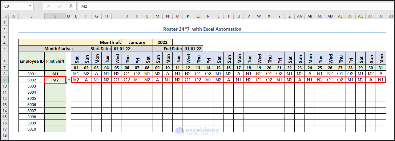
- Select the First Shift for all other employees and the worksheet will automatically give their Shift Roster.
Step 5 – Shift Roster for Different Month
You can create a Shift Roster for different months by just changing the Month and Year.
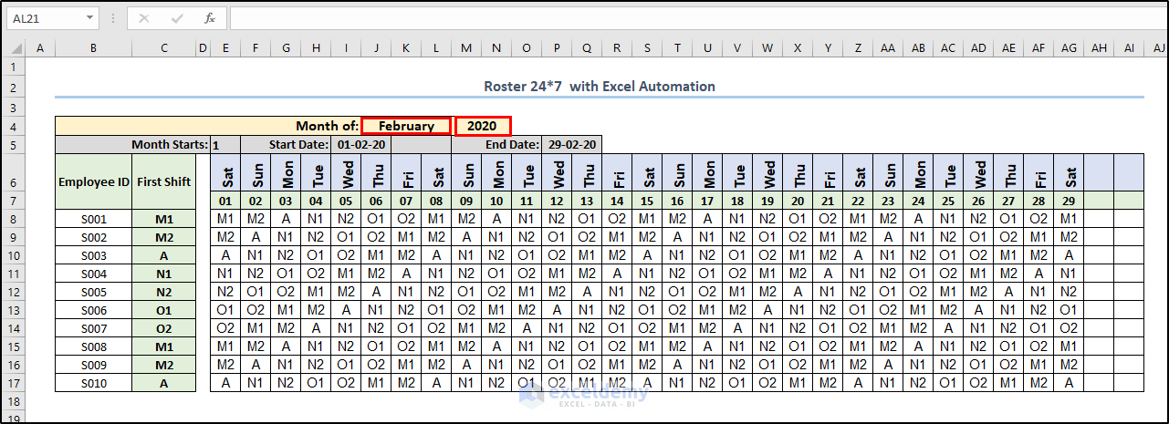
- From the dropdown boxes, change the month to February and the Year to 2020.
And automatically, the spreadsheet will give the Shift Roster for February 2020.
This month has 29 days, and it has been modified accordingly.
Read More: How to Create Monthly Duty Roster Format in Excel
Frequently Asked Questions
1. What information should be included in a shift roster?
A shift roster can include the name of the employee, the date, the start and end time of the shift, the type of shift (e.g. morning, afternoon, night), and any notes or comments (e.g. overtime, training).
2. Can I use Excel to generate automatic alerts or reminders for shift changes?
Yes. You can use VBA code or conditional formatting. For example, you can assign a rule that highlights shifts that have been changed or send an email notification to affected employees.
3. Can I use Excel to track employee attendance or time off?
Yes, you can track employee attendance or time off by adding columns or sheets to the roster and you can use formulas or functions to calculate the total hours worked or missed. You can also use conditional formatting or data validation to indicate absences or holidays.
4. Can I use Excel to create a visual representation of the shift roster?
Yes, you can use Excel to create a visual representation of the shift roster with charts or graphs. For example, you can create a Gantt chart to show the duration and overlap of shifts or a pie chart to show the distribution of shifts by type.
5. How can I protect the shift roster from accidental or intentional changes?
You can protect the shift roster using Excel’s protection features such as password protection, worksheet protection, or workbook protection from accidental or intentional changes. You can also restrict specific cells or ranges from editing or formatting.
Things to Remember
- You should ensure proper formatting for the start and end dates.
- Mention all relevant information about your Shift Roster.
- You can use conditional formatting to highlight any shift that has special characteristics.
- You should check your roster properly before using it.
Download Practice Workbook
You can download this practice workbook.
Download Shift Roaster with Leave Request Template
Related Articles
- How to Create Weekly Duty Roster Format in Excel
- Weekly Meal Planner Template with Snacks
- How to Create Automatic Schedule Generator for Free in Excel
<< Go Back to Roaster Templates | Excel Templates
Get FREE Advanced Excel Exercises with Solutions!


excellent, i want to create a roaster include D1 D2 DN N1 N2 O. This one must rotate full month and continue next month.
for example in January 1st can come dn and february 1st o.
can u create a formula for this?
Hello TH
Thanks for reaching out and sharing your requirements. You wanted a roaster including D1, D2, DN, N1, N2, and O to rotate full month and continue next month.
I am delighted to inform you that I have created a roaster to fulfil your goal. So, follow these:
Return to the sheet, and use the file like the following GIF.
Hopefully, the idea will work for you. I am attaching the solution workbook for better understanding. Good luck.
DOWNLOAD SOLUTION WORKBOOK
Regards
Lutfor Rahman Shimanto
ExcelDemy
Hi Team,
Thanks for the Excel. I need to create a shift for 4 Members Team. The shifts are
Shift A: Monday to Friday- Day shift ( Sat and Sun Week Off)
Shift B: Monday to Friday- Night shift ( Sat and Sun Week Off)
Shift C: Monday ,Tuesday, Wednesday, Saturday, Sunday – Day Shift ( Thursday , Friday Week off)
Shift D: Wednesday , Thursday, Friday – Day Shift , Saturday, Sunday – Night Shift ( Monday and Tuesday Week off)
On Wednesdays All 4 members will Work in 3 persons in Day shift and 1 person in night shift.
Can you please help to create this shift scheduler.
Thanks
Karthick
Hi Karthick
Thank you for reaching out with your inquiry! Designing a shift schedule for a 4-member team roster with diverse shift patterns can be challenging.
Each shift, A, B, C, and D, has a schedule for weekdays, weekends, and special arrangements on Wednesdays. Setting these parameters upfront allows you to assign team members to their shifts more efficiently.
On Wednesdays, all four members are active but in different roles. It would be best if you had a flexible framework to handle this. One idea is to create a dynamic formula that adjusts shift assignments based on the day of the week and specific requirements. This might involve using conditional logic to distribute team members across day and night shifts, ensuring we have enough coverage while using resources effectively.
Don’t forget to explore the resources in the article, including the practice workbook, to gain hands-on experience with building and refining your shift scheduler. Good luck.
Regards
Lutfor Rahman Shimanto
ExcelDemy
Dear Sir Lutfor Rahman Shimanto,
I have also a query regarding on the sample, Instead of using D1,D2,D3,D4,OFF,A1,A2,A3,OFF, is it possible to use just like this only D,D,D,D,OFF,A,A,A,OFF..
Thank you in advance.
Regards,
Eral
Hello ERAL
Good to see you again. You wanted shifts like, Instead of using D1, D2, D3, D4, OFF, A1, A2, A3, OFF, is it possible to use just like this only D, D, D, D, OFF, A, A, A, OFF. Technically, it is impossible without VBA, but I have found a trick to reach your goal. I have used extra spaces in the Settings_Shift_Legend to make the shifts unique.
OUTPUT OVERVIEW
Hopefully, I will like the idea. I have attached the solution workbook to help you understand better; good luck.
Download Solution Workbook
Regards
Lutfor Rahman Shimanto
ExcelDemy
Hi Team,
I need to create a shift for 5 Members Team. The shifts are
Morning- Shift A
Evening- Shift B
Night- Shift C
General- Shift D
Shift Members are 1,2,3,4,5
shift member 1 having week off on Friday & sat
Shift member 2 having week off on Sun & Mon
Shift member 3 having week off on Tue & Wed
shift member 4 having week off on Thu & Fri
Shift member 5 having week off on Sat & Sun
*Shift member 5 do only General & when required Moring shift only.
Can you please help to create this shift scheduler.
Thanks
Shivam
Hello SHIVAM
Thanks for your comment. To create a shift scheduler for a 5-member team with the specified shifts and off days, you can follow these steps:
Here is an example of how you could structure the scheduler:
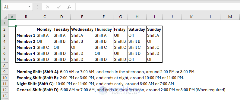
Hopefully, the idea will help you; good luck.
Regards
Lutfor Rahman Shimanto
ExcelDemy
Sometimes before creating the schedule for the next month, we will blast information to the customer service staff for those who want to apply for leave. How do we handle the scheduling formula if there are leave requests for that month?
Hello Agung,
To handle the leave request for next month we updated our existing template. Added a new sheet to enter leave requests. Based on this sheet modified the existing formulas to consider leave request.
You will get a roaster template without leave request:
=IF(AND(INDEX(LeaveRequests!$B$2:$B$11,MATCH(‘Roster 24”7’!$B$8,LeaveRequests!$A$2:$A$11,0),1)<=E$7,INDEX(LeaveRequests!$C$2:$C$11,MATCH('Roster 24''7'!$B$8,LeaveRequests!$A$2:$A$11,0),1)>=E$7), IF(OR($C8=””,E$7=””), “”,IF(D8= “”,C8, INDEX(Settings_Shift_Legend,IF(MATCH(RIGHT(D8,2),Settings_Shift_Legend,0)+1>COUNTA(Settings_Shift_Legend),1,MATCH(RIGHT(D8,2),Settings_Shift_Legend,0)+1))))&”- On leave”, IF(OR($C8=””,E$7=””), “”,IF(D8= “”,C8, INDEX(Settings_Shift_Legend,IF(MATCH(RIGHT(D8,2),Settings_Shift_Legend,0)+1>COUNTA(Settings_Shift_Legend),1,MATCH(RIGHT(D8,2),Settings_Shift_Legend,0)+1)))))
Here is the formula to show leave requests:
=IF(AND(INDEX(LeaveRequests!$B$2:$B$11,MATCH(‘Roster 24”7’!$B$8,LeaveRequests!$A$2:$A$11,0),1)<=E$7,INDEX(LeaveRequests!$C$2:$C$11,MATCH('Roster 24''7'!$B$8,LeaveRequests!$A$2:$A$11,0),1)>=E$7), IF(OR($C8=””,E$7=””), “”,IF(D8= “”,C8, INDEX(Settings_Shift_Legend,IF(MATCH(RIGHT(D8,2),Settings_Shift_Legend,0)+1>COUNTA(Settings_Shift_Legend),1,MATCH(RIGHT(D8,2),Settings_Shift_Legend,0)+1))))&” – Leave Req”, IF(OR($C8=””,E$7=””), “”,IF(D8= “”,C8, INDEX(Settings_Shift_Legend,IF(MATCH(RIGHT(D8,2),Settings_Shift_Legend,0)+1>COUNTA(Settings_Shift_Legend),1,MATCH(RIGHT(D8,2),Settings_Shift_Legend,0)+1)))))
Download the Excel File: 24×7 Shift Roaster Template with Leave Requests
Regards
ExcelDemy
Good Afternoon Gentlemen
I need to create a roster following this criteria
Duty roster covering the period from January 1, 2025, to December 31, 2025.
8 employees covering 3 shifts S1 7am to 4pm S2 1pm to 10pm S3 10pm to 7am with a 5/2 work schedule and 24/7 coverage
Hello Khaled,
To create a 24/7 roster from January 1, 2025, to December 31, 2025, with 8 employees covering 3 shifts (S1: 7 AM-4 PM, S2: 1 PM-10 PM, S3: 10 PM-7 AM) and a 5/2 schedule:
Define the Roster: Use a table in Excel with dates in rows and employees’ names in columns.
Set Shifts: Assign shifts systematically, rotating employees to cover all shifts.
Automate: Use formulas (like MOD) to cycle shifts and conditional formatting for visual clarity.
Validate Coverage: Check all shifts are filled across weeks for 24/7 operation.
Regards,
ExcelDemy
Hi
I need the formula for one day off and 8 technicians with 3 shifts daily
Hello Aous Ymani,
To assign 8 technicians across 3 shifts per day with one day off per technician, you can use a rotating pattern in Excel. Here’s a basic idea:
Define the shifts: Morning (M), Afternoon (A), Night (N), and Off (O).
Create a pattern like this over a few days:
Day 1: M, A, N, O, M, A, N, O
Day 2: A, N, O, M, A, N, O, M
Day 3: N, O, M, A, N, O, M, A
Use a formula like this to rotate shifts across days (assuming A2 has Day 1 pattern and downwards):
=INDEX({“M”,”A”,”N”,”O”}, MOD(ROW()+COLUMN()-2,4)+1)q
You can adapt this to a full weekly/monthly schedule.
Regards
ExcelDemy
Can anyone help me build one, our rosters work from the 26th of a previous month till the 25th of the current month, also, our shift work a bit different, for example 1 person will work D,D,D,N,N,X,X. D being dayshift,N being nightshift and x being off days and then it repeats itself, but i want to be able to to change my requirements per shift and it adjust all employees shifts based on that.
i would greatly appreciate any help
Hello Ryan,
For your setup, where the roster runs from the 26th of the previous month to the 25th of the current month, you’ll need to adjust the date formulas in the template so the start date is always the 26th, and the end date is the 25th of the next month.
For the repeating pattern (like D, D, D, N, N, X, X), you can set up a “pattern” input cell or row for each employee (or as a master pattern), and then use formulas to repeat that pattern across the days.
If you want to change the pattern and have it auto-update for all employees, you can use a single reference pattern row and have each employee’s shift row pull from that, repeating every 7 days.
If you’d like, I can walk you through the formulas or even share a sample file. Let me know your preferred shift patterns and how many employees you have, and I can help you build a customized template!
Regards
ExcelDemy
Hi shamima
thats great thank you, i would appreciate your assistance, we have a few different sites with employees ranging from 1 dayshift and 1 night shift to 4 day shift and 4 nightshift, so i would like scalablity built into the roster if possible.
I would love a sample roster aswell and if you can explain to me or help me setup the pattern rows
Hello Ryan,
Thank you for the follow-up! Based on your needs—multiple sites with varying numbers of day and night shift employees (from 1 to 4) you can prepare a scalable Excel roster template where:
Roster Dates Setup:
1. In Row 1 (starting from Column B), enter the dates from the 26th of the previous month to the 25th of the current month.
2. Use a formula like this in cell B1:
=DATE(2025,6,26)
3. Then drag across 30 cells to reach the 25th of the next month.
Master Shift Pattern:
1. In a row (e.g., Row 3), input the repeating 7-day pattern: D, D, D, N, N, X, X
2. Use this formula in Row 4 for each date column (starting from B4):
=INDEX($B$3:$H$3,MOD(COLUMN()-COLUMN($B$3),7)+1)
3. This will repeat the pattern every 7 days.
Apply to Employees:
1. Copy Row 4 for each employee’s row to apply the same pattern.
2. If you want each employee to start on a different day in the cycle, adjust the MOD(…)+1 portion accordingly.
Scalability for Multiple Sites:
1. You can group employees by site using separate blocks or color codes.
2. Just replicate the employee section and change headers for each site.
3. To scale up or down, simply copy or delete rows as needed.
You’ll be able to adjust the number of employees per site easily, thanks to dynamic formulas.
Regards
ExcelDemy
Good Morning Shamina
If you can assist me. I need to do a roster per month for 35 employees
5-day shifts on, 3-days off 5-night shift on 3-days off.
everyday there must be 15 on day shift and 9 on night shift.
Regards
Hannes
Hello Hannes,
Good morning! Yes, I can definitely assist you with that.
Step-by-Step Guide to Build the 24×7 Shift Roster in Excel:
Step 1: Set Up the Date Headers
1. In Row 1 (starting from B1), enter all the dates for the month horizontally (e.g., B1:AF1 for a 31-day month).
2. Format them as dd-mmm.
Step 2: List Employees Vertically
In Column A (starting from A2), list all 35 employee names (e.g., A2:A36).
Step 3: Define Shift Codes
Use the following codes:
D = Day shift
N = Night shift
O = Off
Step 4: Create Rotating Pattern
In another sheet or helper table, define a base pattern (e.g., 5D, 3O, 5N, 3O = 16-day cycle). Repeat this pattern across the month for each employee, staggered so shifts rotate evenly.
Example for Employee 1:
D, D, D, D, D, O, O, O, N, N, N, N, N, O, O, O …
Shift each subsequent employee’s pattern by a few days to ensure:
No overcrowding on the same shift
Balanced 15 Day / 9 Night coverage
Step 5: Use Formulas to Apply Patterns
Use Excel formulas like =INDEX() or =OFFSET() to fill in shifts for each day, repeating the 16-day cycle across the month.
Example formula for B2:
=INDEX($Z$2:$AO$2,MOD(COLUMN(B2)-2,16)+1)
Where Z2:AO2 contains the 16-day pattern for that employee.
Step 6: Count Shifts Per Day
Below the roster table (e.g., row 38+), insert formulas to count:
How many “D” per day:
=COUNTIF(B2:B36, “D”)
How many “N” per day:
=COUNTIF(B2:B36, “N”)
Use conditional formatting to highlight if the count isn’t 15 (for day) or 9 (for night).
Step 7: Optional – Add Conditional Formatting
Use color coding:
Green for “D”
Blue for “N”
Gray for “O”
This improves readability.
Regards
ExcelDemy
Hello Team,
Thank you for such a detailed excel explanation.
I have a requirement and need your help there.
1. We have to create a roaster for 10 members , with 3 shifts – Morning, day and Afternoon , Also there will be on call for 1 person and that person will not be from morning shift
2. 2 person can never do morning shifts so they will always be in day and afternoon
3. Vacations will be there which we will update and roster will update as per that
Need your kind help on this
Hello Saptarshi Chakraborty,
Thank you for your thoughtful feedback and detailed requirements! You can adapt the same automation process shown in our article to meet your case:
Three shifts + On-Call: Keep the Morning/Day/Afternoon setup from the article, then add an extra “On-Call” row below the roster. Use a simple formula to rotate through your team while excluding the Morning person each day, so the on-call is always different.
Two members never on Morning: In the Settings sheet, make a second shift legend that leaves out the Morning option. Apply the article’s step-4 formula to those two people but point it to the no-morning legend. This way, their rotation cycles only through Day and Afternoon.
=IF(E$7=””,””,
LET(mrng,$E$8,
pool,FILTER(People,People<>mrng),
INDEX(pool,1+MOD(COLUMNS($E$7:E$7)-1,ROWS(pool)))
)
)
Vacations/Leave: The template already supports adding leave codes. You can log vacation days directly in the roster (using an “L” code) or download the linked template with a Leave Request sheet. Either way, the roster automatically updates around absences.
=IF(OR($C8=””,E$7=””),””,
IF(D8=””,
C8,
INDEX(Settings_Shift_Legend_NoM,
IF(MATCH(D8,Settings_Shift_Legend_NoM,0)+1>COUNTA(Settings_Shift_Legend_NoM),
1,
MATCH(D8,Settings_Shift_Legend_NoM,0)+1))))
This approach follows the same formulas and named ranges we used in the tutorial, just with slight adjustments to handle your custom rules. If you’d like, we can prepare a sample workbook with your 10 names and the two “no-morning” members pre-set.
Regards,
ExcelDemy
Hello Shamima,
I cant thank you enough for all the prompt support you had shown in this conversation.
I have one issue here, which need your expert advice , Our roaster remain same through out the week and only changes every week.
and its Mon – Fri day only and not 24X7 . May i know what changes i need to do in your program for that
Hello,
You can make the roster Mon–Fri only and keep the same assignments all week (then rotate next week) with two small tweaks:
1) Make the Date column weekdays only
In A2, use:
=WORKDAY(A$2, ROWS($A$2:A2)-1)
(Or put your first Monday in A2, then fill this down. It will list only business days—no Sat/Sun.)
2) Switch the rotation from “daily” to “weekly”
In each assignment formula, replace the daily counter with a week index:
wk, QUOTIENT(ROWS($A$2:A2)-1,5)+1
Then use wk inside MOD() so the same people repeat across Mon–Fri and change only next week.
Morning (B2)
=LET(
names, People,
allow, AllowMorning,
d, $A2,
wk, QUOTIENT(ROWS($A$2:A2)-1,5)+1,
notOnLeave, COUNTIFS(Vacations!$A:$A,names,Vacations!$B:$B,d)=0,
pool, FILTER(names,(allow=”Yes”)*notOnLeave),
IF(ROWS(pool)=0,””, INDEX(pool, 1+MOD(wk-1, ROWS(pool)))))
Day (C2)
=LET(
names, People,
d, $A2,
wk, QUOTIENT(ROWS($A$2:A2)-1,5)+1,
mrng, $B2,
notOnLeave, COUNTIFS(Vacations!$A:$A,names,Vacations!$B:$B,d)=0,
pool, FILTER(names,(names<>mrng)*notOnLeave),
IF(ROWS(pool)=0,””, INDEX(pool, 1+MOD(wk-1, ROWS(pool)))))
Afternoon (D2)
=LET(
names, People,
d, $A2,
wk, QUOTIENT(ROWS($A$2:A2)-1,5)+1,
mrng, $B2,
dayp, $C2,
notOnLeave, COUNTIFS(Vacations!$A:$A,names,Vacations!$B:$B,d)=0,
pool, FILTER(names,(names<>mrng)*(names<>dayp)*notOnLeave),
IF(ROWS(pool)=0,””, INDEX(pool, 1+MOD(wk-1, ROWS(pool)))))
On-Call (E2)
=LET(
names, People,
d, $A2,
wk, QUOTIENT(ROWS($A$2:A2)-1,5)+1,
mrng, $B2,
dayp, $C2,
aftn, $D2,
notOnLeave, COUNTIFS(Vacations!$A:$A,names,Vacations!$B:$B,d)=0,
pool, FILTER(names,(names<>mrng)*(names<>dayp)*(names<>aftn)*notOnLeave),
IF(ROWS(pool)=0,””, INDEX(pool, 1+MOD(wk-1, ROWS(pool)))))
The same Morning/Day/Afternoon/On-Call apply for the whole week, then rotate once per new week; weekends are automatically skipped. Vacations still work—if someone is on leave on a given day, the formula substitutes from the remaining pool.
Regards,
ExcelDemy
Hello Shamima,
Thank you very much for your reply , I really appreciate your prompt response, I am trying to prepare it but may be I am missing something so the results are not coming. Can you please help me with the pre-set as you mentioned.
Hello again!
Since setting up all the formulas by hand can be tricky, I’ve prepared a pre-set file for you.
[Download the roster template here]
What’s included:
Settings sheet: 10 members listed, with “AllowMorning” so two members can be excluded from Morning shifts.
Vacations sheet: Add names + dates, and the roster updates automatically.
Roster sheet: Already filled with formulas for Morning, Day, Afternoon, and On-Call (On-Call never overlaps with Morning).
Just replace the placeholder names with your actual team members, mark the two “No” under Morning, and enter vacation dates as needed. The rest will auto-update.
Regards,
ExcelDemy