How to Create an Automatic Schedule Generator in Excel (Easy Steps)

Step 1 – Prepare the Dataset

Dataset Selection:
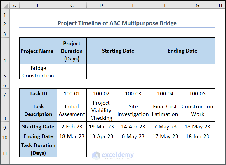
- Assume we have a dataset named “Project Timeline of ABC Multipurpose Bridge.” However, feel free to use any dataset that suits your needs.

How to Create Automatic Schedule Generator for Free in Excel

Pre-processing Tasks:

- Before diving into today’s topic, perform some pre-processing tasks:
  - Sort the project’s starting and ending dates.
  - Calculate task durations.
  - Determine the overall project duration.

Formulas:
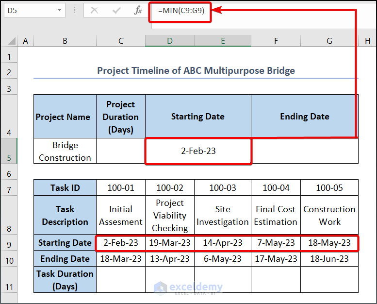
- In cell D5, enter the following formula:

=MIN(C9:G9)

⚡Formula Breakdown

- - Here C9:G9 represent the Starting Date of the different tasks in the construction project.
  - The MIN function finds the earliest starting date.
  - Output: 2-Feb-23

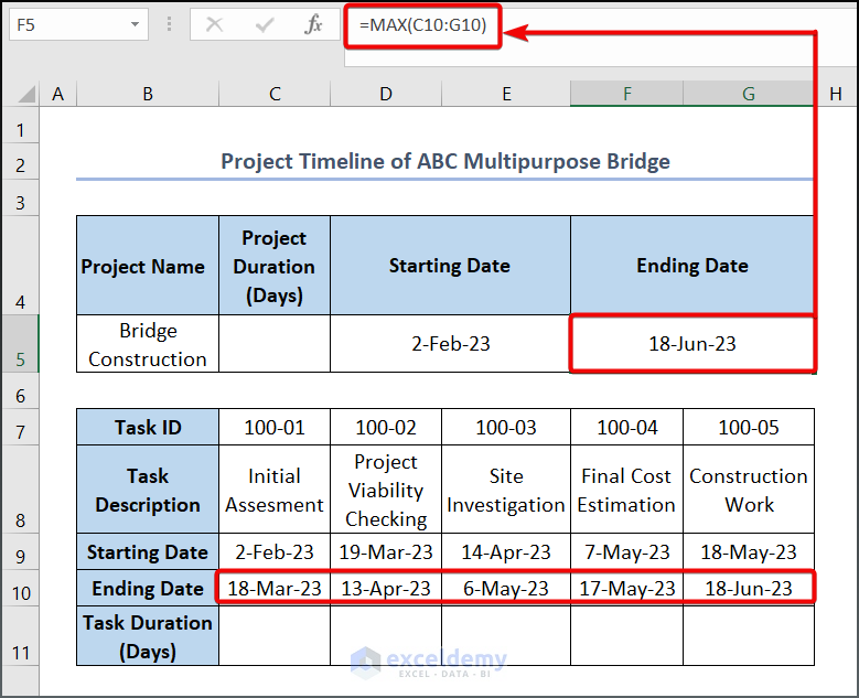
- To find the Ending Date of the project, use the MAX function:
- Enter the following formula in cell F5.

=MAX(C10:G10)

⚡Formula Breakdown

- - C10:G10 represents the ending dates of the project tasks.
  - Output: 18-Jun-23

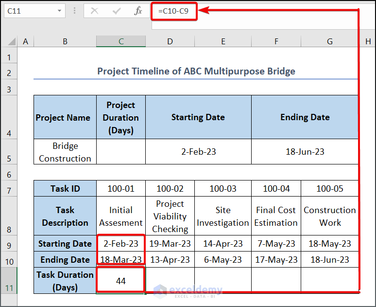
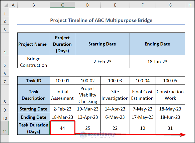
- To calculate the duration of each task, enter the following formula in cell C11:

=C10-C9

- - C9 and C10 represent the starting and ending dates of each task, respectively.

- Drag the Fill Handle tool to populate other values.

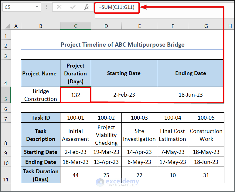
- To SUM up the task durations, enter the following formula in cell C5:

=SUM(C11:G11)

- - C11:G11 represents the time duration of each task from Feb 2nd to June 18th.

Step 2 – Create the Automatic Schedule Generator

Input Dates:
- Input “2-Feb-2023” and “3-Feb-2023” in cells B12 and B13, respectively.
- Select these cells and drag the Fill Handle from B12 to B148 to generate other dates.

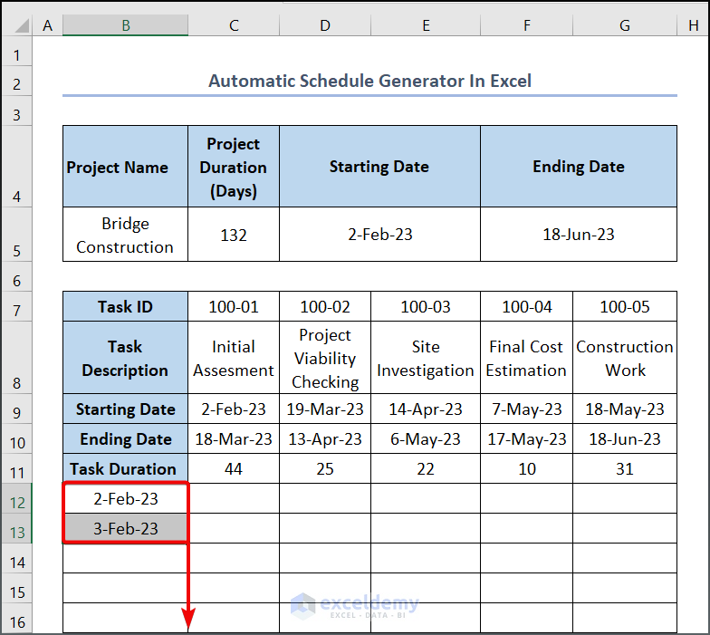
See the GIF attached below to get a visual demonstration of it.

Formula for Schedule Generation:
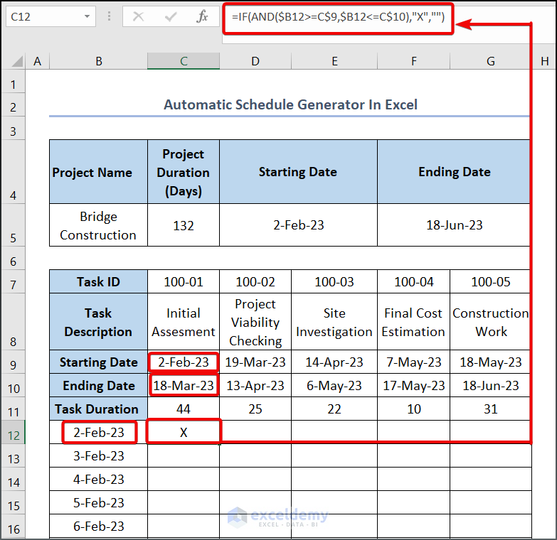
- In cell D5, enter the following formula:

=IF(AND($B12>=C$9,$B12<=C$10),"X","")

⚡ Formula Breakdown:

- - This formula checks if the date in B12 falls within the project’s start and end dates (C9 and C10).
  - If true, it returns “X”; otherwise, the cell remains empty.

See the output as given below.

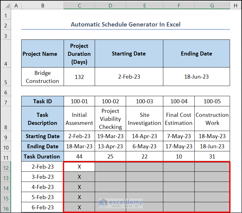
Output Visualization:
- Drag down the formula in the C12:G148 range to see the complete schedule.

Step 3 – Highlight Occupied Days

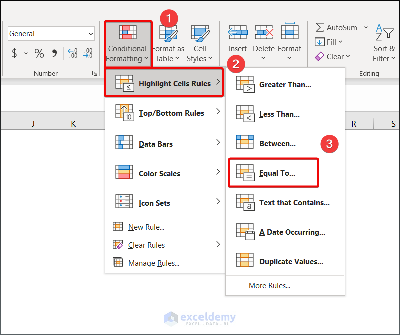
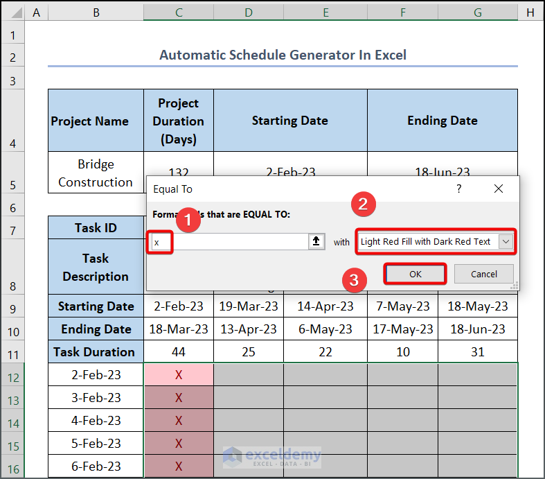
Aesthetic Enhancement:
- Select all cells in the C12:G148 range.

- Go to Home > Conditional Formatting > Highlight Cells Rules > Equal To.

- Enter X and choose Light Red Fill with Dark Red Text (or your preferred style).
- Click OK.

- Now see the output as given below.

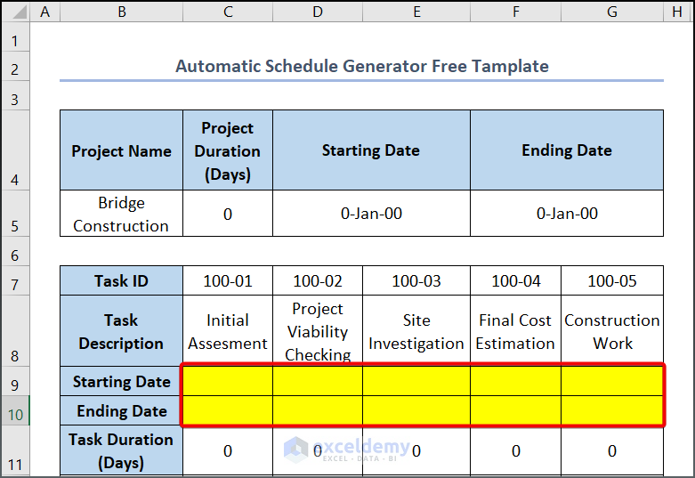
Free Template: Ready to Use

Use the ready-made template provided in the Excel file. Simply input the starting and ending dates for each task in the highlighted cells. Adjust the dates in Column B according to your project duration.

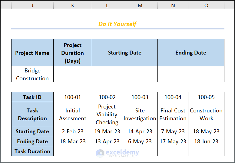
Practice Section

We have provided a Practice section on the right side of the sheet so you can practice yourself. Please make sure to do it yourself.