How to Create an Attendance Roster in Excel (with Easy Steps)

In this article, I will show you how to create an attendance roster in Excel. As we know, Excel is a very handy tool for keeping track of employees’ daily attendance and different sorts of leaves. Here, I will show you all the steps on how we can make a sample attendance roster in Excel where we can keep records of all of the parameters mentioned above. So, let’s get started.

How to Create an Attendance Roster in Excel: with Easy Steps

Here, I will show you all the necessary steps for making a simple attendance roster for a company. In this roaster file, I will keep track of the following parameter.

Daily Attendance (P)
Leave (L)
Half-Day (HD)
Sick Leave (SL)
Casual Leave (CL)
Training Leave (TL)
National Leave (NL)
Festive Leave (FL)
Maternity Leave (ML)
Earned Leave (EL)

In this article, the record will be shown for an imaginary company named “Multivita International Limited”. Here, the company will have two weekly holidays (Saturday and Sunday). By the end of the month, this file will also provide a monthly attendance summary. Now, let’s jump into the steps for creating this roaster attendance file.

Step 1: Giving a Title to Roster Sheet

In this step, we will set a title for the roster sheet. To do that, follow the steps below.

In the very first step, we need to open a fresh Excel Workbook.
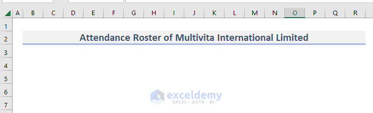
Next, we have to take some cells from one of the top rows and merged those cells into one. I have taken B2:R2 and merged them.

Now, give a suitable title to it. I have given the name “Attendance Roster of Multivita International Limited”. Then modify the formatting of the cell to make it more attractive and elegant.

Step 2: Inserting Column Headers

In the 2nd step, we will be inserting column headers. To do that, follow the steps given below.

In this step, we need to insert the column headers in the worksheet. Usually, in an attendance roaster, the column headers include Year, Month, Date, Employee ID, Employee Name, and Weekdays.

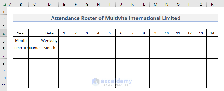
Here, due to the image size limitation, I am showing you only the first two weeks of dates. But, in the provided file, you will see the entire dates of a month.
Now, modify the formatting of each column header to make it more attractive.

Step 3: Assigning Conditional Formatting

In the 3rd step, we will apply conditional formatting to highlight the weekend holidays. To do that, follow the steps below.

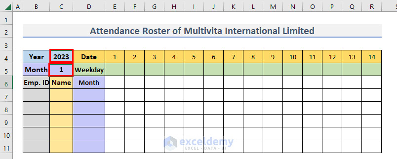
Now, we need to assign conditional formatting to the cells so that the weekly holidays can be easily distinguished. To do that, let’s take a month such as January 2023 for illustration purposes.

Now, to automatically determine the weekdays for corresponding dates in a month, use the following formula in cell E5.

=SWITCH(WEEKDAY(DATE($C$4,$C$5,E$4),1),1,"Sun",2,"Mon",3,"Tues",4,"Wed",5,"Thu",6,"Fri",7,"Sat")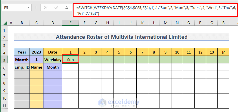

How Does the Formula Work?

In this formula, the DATE function is used to extract the date using different cell values. Then this date value is inserted as an argument in the WEEKDAY function to determine the weekday of this date. As the WEEKDAY function returns the weekday in numbers (1 for Sunday, 2 for Monday, and so on), we have used the SWITCH function to display the weekday directly as Text.

Now, use the Fill Handle to autofill the rest of the weekdays.

Now, to automatically insert the name of the month, use the following formula in the Month column.

=SWITCH($C$5,1,"January",2,"February",3,"March",4,"April",5,"May",6,"June",7,"July",8,"August",9,"September",10,"October",11,"November",12,"December")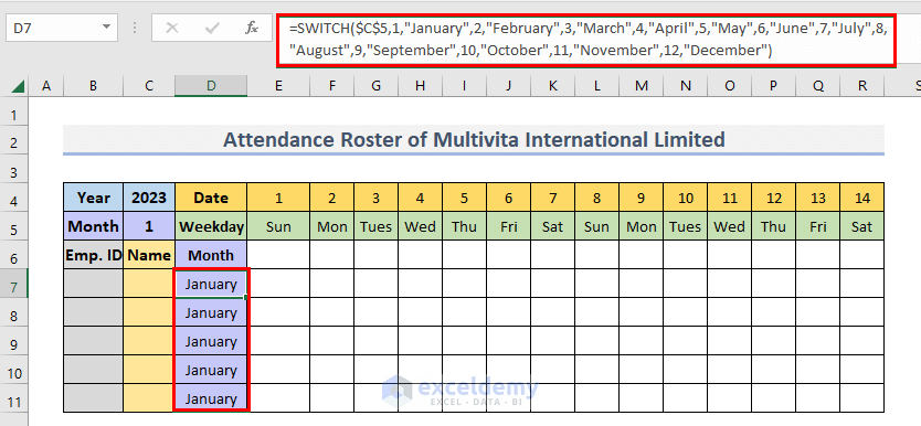

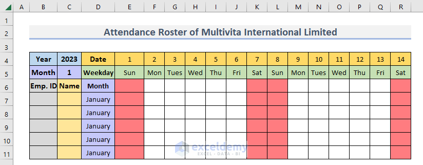
Now, in order to apply a different background color to the weekend columns, first select all the cells in the data table, then in the Home tab, go to Conditional Formatting >> New Rule.

Now, from the popped-up dialogue box, select Use a formula to determine which cells to format, and in the formula box, write down the following formula. Finally, set the formatting according to your choice and then click

=OR(E$5="Sun",E$5="Sat")

As a result, you will see that the weekends are being highlighted in your chosen color.

Step 4: Addition of Monthly Assessment Criteria

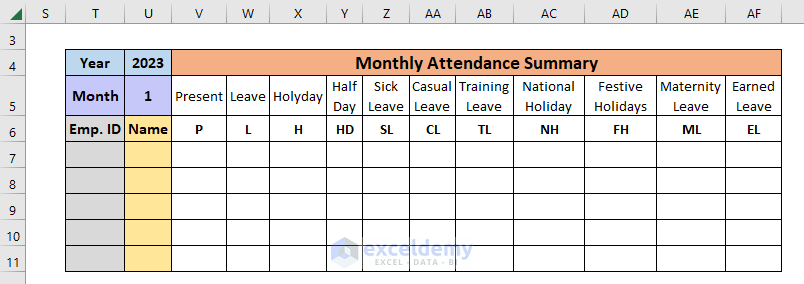
Here, we will add a table that will give a summary of every employee’s attendance. To do that, follow the steps below.

Here, we will add another table that will summarise the monthly assessment for all the employees. The summary table will be like this.

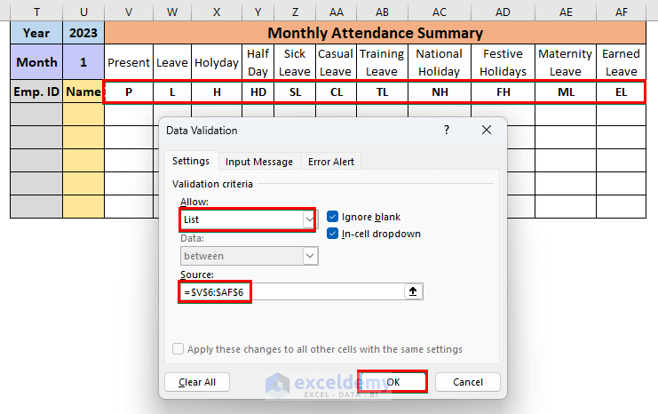
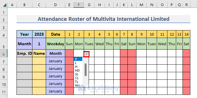
Now, we will add the Data Validation feature to all the cells so that we can choose from a dropdown menu while inserting attendance To do that, first, select all the cells where the attendance will be inserted, and then go to the Data tab and click on Data Validation.

Now, in the dialogue box, select List as Validation criteria, and as a source, select the cells from the Monthly Attendance Summary that contain the values which you want to insert. Finally, click on OK.

As a result, you will see that if you click any cell, a list will be available from which you can choose the value which you want to insert.

Now, go to the Monthly Attendance Summary Here, we will write a formula to count the number of days in a month an employee has been present, on leave, or other kinds of absences. To do that, write the formula in cell V7 which includes the COUNTIF function.

=COUNTIF($E7:$R7,V$6)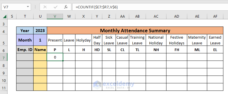

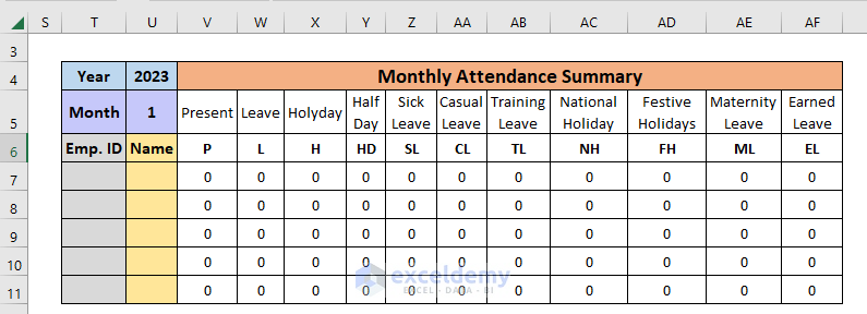
Now, use the Fill Handle to apply the formula in other cells in this table.

Step 5: Filling up Roster

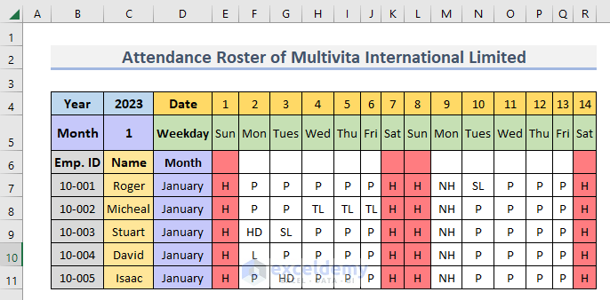
In the final steps, we will insert some random data in the roster to display a sample final result.

In this step, we will fill the roaster to display how would the roaster look like when all the necessary data you want to insert. Hence, we inserted some random data here.

As a result, the summary table will look like this.

In this way, we can create a simple yet productive attendance roster in Excel.

Things to Remember

In the sample dataset, I have taken only 1st two weeks. But in the final Excel file, we have designed the table for an entire month.

Download Practice Workbook

Download this practice workbook to exercise while you are reading this article.

Attendance Roster.xlsx

Conclusion

That is the end of this article regarding how to create an attendance roster in Excel. If you find this article helpful, please share this with your friends. Moreover, do let us know if you have any further queries.

<< Go Back to Roaster Templates | Excel Templates

Get FREE Advanced Excel Exercises with Solutions!