Example 1 – Using VLOOKUP Between Two Sheets in the Same Excel Workbook
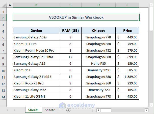
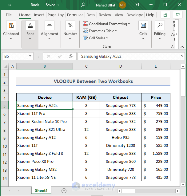
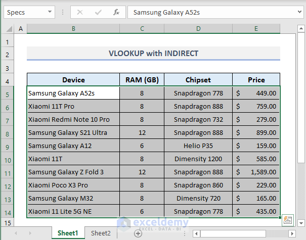
In the following picture, Sheet1 is representing some specifications of a number of smartphone models.
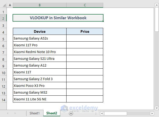
And here is Sheet2, where only two columns from the first sheet have been extracted. In the Price column, we’ll apply the VLOOKUP function to get the prices of all devices from Sheet1.
- The required formula in the first output Cell C5 in Sheet2 will be:
=VLOOKUP($B5,Sheet1!$B$5:$E$14,4,FALSE)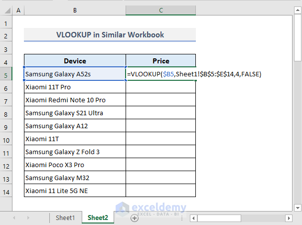
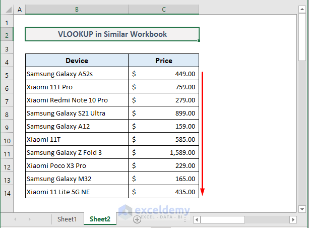
- Press Enter and you’ll get the price of the first smartphone device extracted from Sheet1.
- Use Fill Handle to autofill the rest of the cells in Column C.
Read More:How to Use VLOOKUP Formula in Excel with Multiple Sheets
Example 2 – Using VLOOKUP Between Two Sheets in Different Workbooks
The following primary data table is in a workbook named Book1.
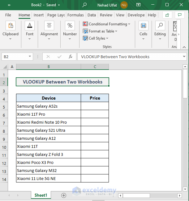
Here is another workbook named Book2 that will represent the output data extracted from the first workbook.
- In the second workbook, the required formula in the first output Cell C5 will be:
=VLOOKUP(B5, [Book1.xlsx]Sheet1!$B$5:$E$14,4, FALSE)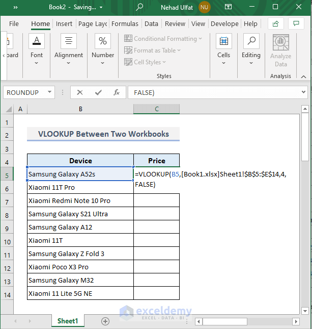
- After pressing Enter and auto-filling the rest of the cells in the Price column, you’ll get all the output data right away as shown in the picture below.
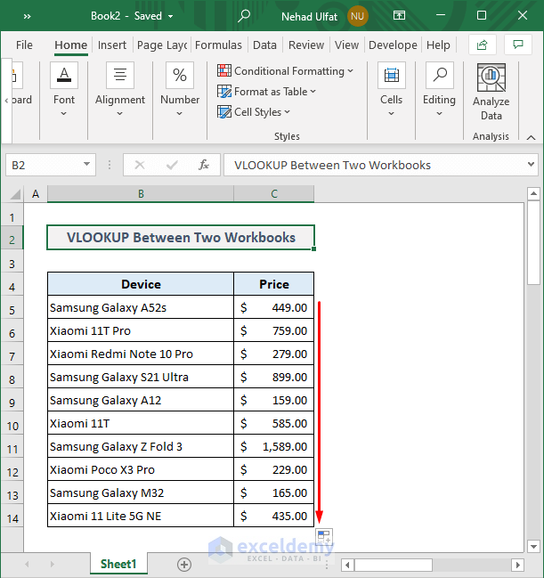
Note: While extracting data from a different workbook, both workbooks have to be open. Otherwise, the formula won’t work and will return a #N/A error.
Example 3 – IFERROR with VLOOKUP Across Two Worksheets in Excel
In the example, the smartphone device in Cell B5 is not available in Sheet1. So, in the output Cell C5, the VLOOKUP function should return an error value. We’ll now replace the error value with a customized Not Found.
- The required formula in Cell C5 should be now:
=IFERROR(VLOOKUP(B5,Sheet1!B5:E14,4,FALSE),"Not Found")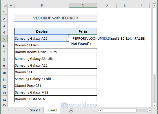
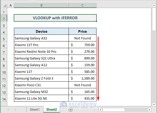
- After pressing Enter and auto-filling the entire column, we’ll get the following outputs.
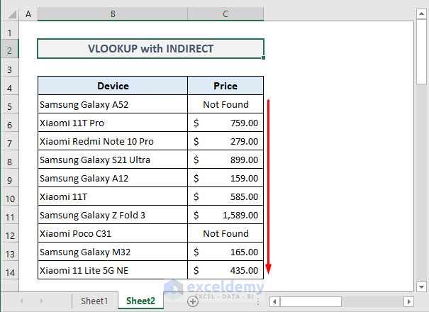
Example 4 – Combining INDIRECT with VLOOKUP for Two Sheets in Excel
- Select the range of cells B5:E14 and go to the Name Box, then input a name. We named the range as Specs.
- In Sheet2, the required formula in the output Cell C5 will be:
=IFERROR(VLOOKUP(B5,INDIRECT("Specs"),4,FALSE),"Not Found")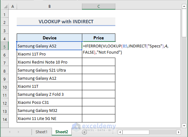
- Here’s the result after using AutoFill.
Download the Practice Workbook
You May Also Like to Explore
- 10 Best Practices with VLOOKUP in Excel
- 7 Practical Examples of VLOOKUP Function in Excel
- How to Use Dynamic VLOOKUP in Excel
- Transfer Data from One Excel Worksheet to Another Automatically with VLOOKUP
- How to Make VLOOKUP Case Sensitive in Excel
- VLOOKUP from Another Sheet in Excel
- How to Remove Vlookup Formula in Excel
- How to Apply VLOOKUP to Return Blank Instead of 0 or NA
- How to Hide VLOOKUP Source Data in Excel
- How to Copy VLOOKUP Formula in Excel
<< Go Back to VLOOKUP Between Worksheets | Excel VLOOKUP Function | Excel Functions | Learn Excel
Get FREE Advanced Excel Exercises with Solutions!

I need to lookup a meter number in column A from one table, find that same meter number in column A from another table and return the reading value in column B from the second table. If there is no match for the meter number, then return a blank for that cell. How do I do that? Here is a partial list of the tables. Help please
Table 1 Table 2
Meter Value Meter Value
160404015 457 160404015 457
160404016 737 160404016 737
160404017 386
160404019 734 160404019 737
160404021 1551 160404021 1852
Use the following formula =IFERROR(VLOOKUP(B5,D5:E9,2,FALSE),””)
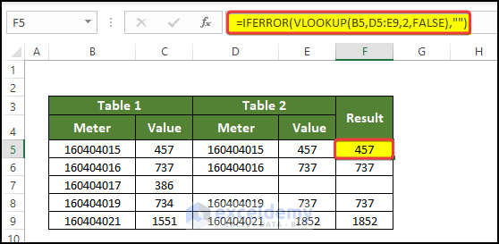
Your given sample table is stored in column B: D. And this VLOOKUP function will look for the value of cell B5(table 1) in the first column on table 2, and then using that position, will return the meter reading from the E column. And it will return blank if there isn’t any meter reading.