Method 1 – Using VLOOKUP Function to Transfer Data from One Worksheet of the Same Workbook to Another
Steps:
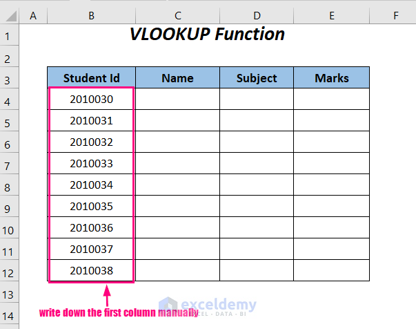
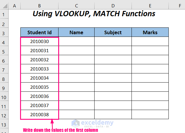
Using the VLOOKUP function, you need to look up values and, for this reason, copy or write down the first column’s data manually.
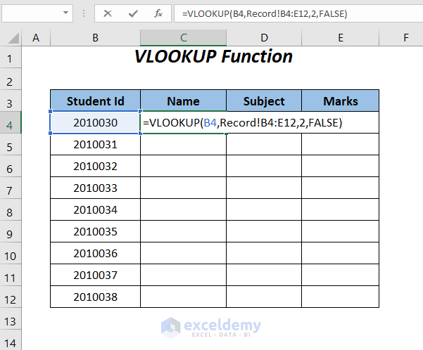
➤ Type the following formula in cell C4.
=VLOOKUP(B4,Record!B4:E12,2,FALSE)B4 is the lookup value, Record!B4:E12 is the data range of the Record sheet, 2 is the column number for the students’ names, and FALSE is for an exact match.
➤ Press ENTER and drag down the Fill Handle tool.
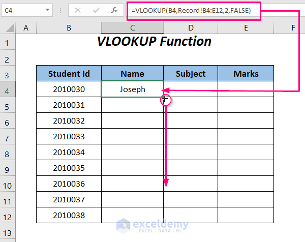
You will get all the names from the source dataset.
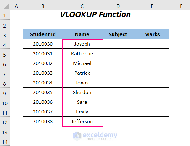
Use the following two formulas to transfer the data from the Subject and Marks columns to this sheet.
=VLOOKUP(B4,Record!B4:E12,3,FALSE)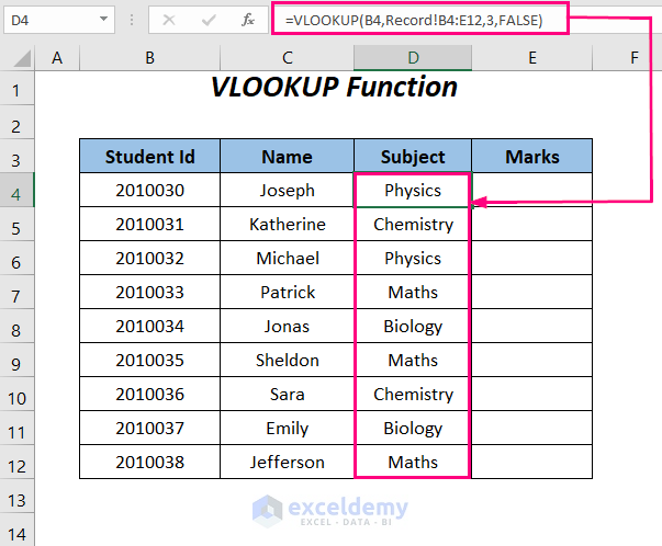
=VLOOKUP(B4,Record!B4:E12,4,FALSE)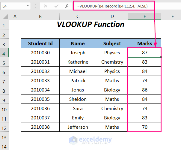
Method 2 – Using VLOOKUP Function with Named Range
Steps:
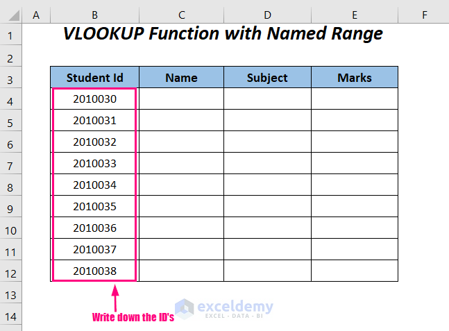
To work with the VLOOKUP function, copy or write down the first column’s data in the Student ID column.
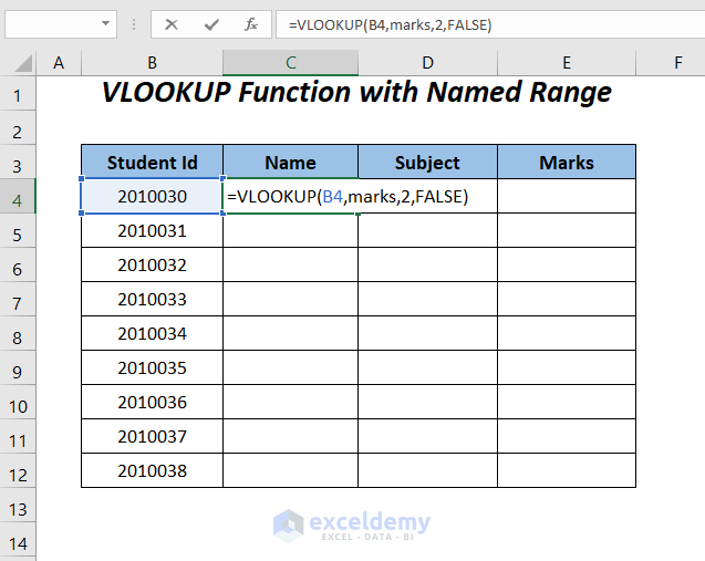
➤ Type the following formula in cell C4.
=VLOOKUP(B4,marks,2,FALSE)B4 is the lookup value, marks is the named range of the Record sheet, 2 is the column number for the students’ names, and FALSE is for an exact match.
➤ Press ENTER and drag down the Fill Handle tool.
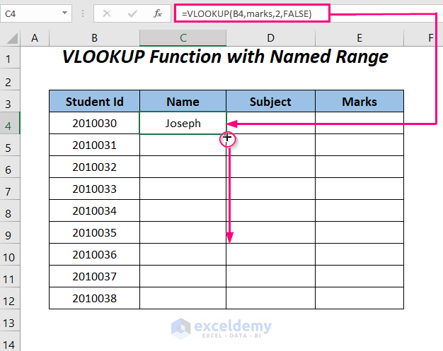
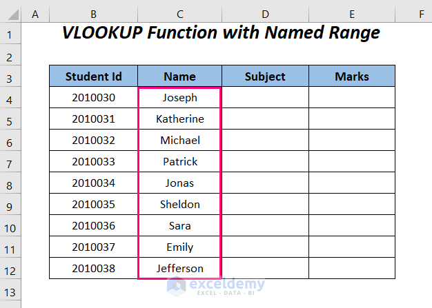
You will have the students’ names corresponding to the IDs in the Name column.
Apply the following formulas to extract the subjects and marks of the students.
=VLOOKUP(B4,marks,3,FALSE)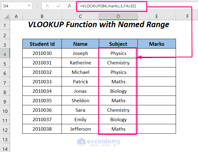
=VLOOKUP(B4, marks,4, FALSE)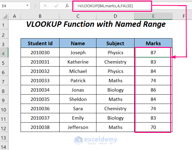
Method 3 – Using VLOOKUP and MATCH Functions to Transfer Data from One Excel Worksheet to Another Automatically
Steps:
To use the VLOOKUP function, we need to look up values, so you must copy or write down the first column’s data manually.
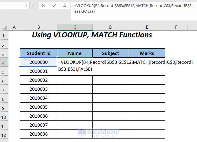
➤ Type the following formula in cell C4.
=VLOOKUP(B4,Record!$B$3:$E$12,MATCH(Record!C$3,Record!B$3:E$3),FALSE)B4 is the lookup value, and Record!B3:E12 is the data range of the Record sheet.
- MATCH(Record!C$3, Record!B$3:E$3) becomes
MATCH(“Name”, Record!B$3:E$3) → MATCH will give the column index number of the header “Name” in the range of headers B$3:E$3 in the Record sheet.
Output → 2
- VLOOKUP(B4,Record!$B$3:$E$12,MATCH(Record!C$3,Record!B$3:E$3),FALSE) becomes
VLOOKUP(2010030, Record!$B$3:$E$12,2, FALSE) → returns the name of the student for the ID 2010030
Output → Joseph
➤ Press ENTER and drag down the Fill Handle tool.
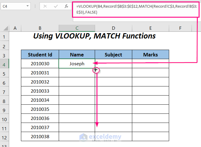
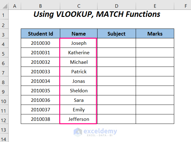
You will have the student’s names in the Name column.
Use the following two formulas to move the data from the Subject and Marks columns to this sheet.
=VLOOKUP(B4,Record!$B$3:$E$12,MATCH(Record!D$3,Record!B$3:E$3),FALSE)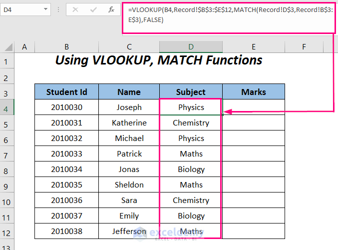
=VLOOKUP(B4,Record!$B$3:$E$12,MATCH(Record!E$3,Record!B$3:E$3,0),FALSE)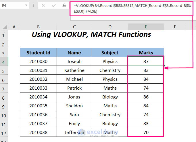
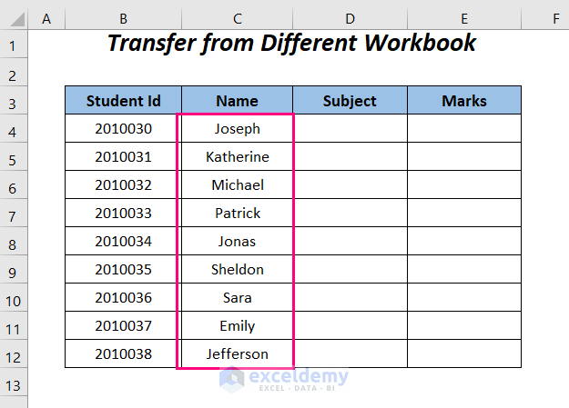
Method 4 – Using VLOOKUP Function to Transfer Data from One Worksheet to Another Workbook Automatically
Steps:
Apply the following formula in cell C4.
=VLOOKUP(B4,'C:\Users\Mima\Downloads\[Source Data.xlsx]Data'!$B$4:$E$12,2,FALSE)B4 is the lookup value, $B$4:$E$12 is the data range of the Data worksheet in the Source Data.xlsx workbook, and you have declared the path of this file preceding the file name.
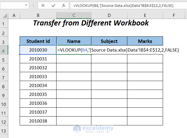
➤ Press ENTER and drag down the Fill Handle tool.
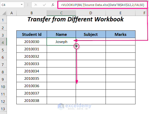
Get all of the names of the students in the Name column.
Use the following two formulas to have the data for the Subject column and the Marks column.
=VLOOKUP(B4,'C:\Users\Mima\Downloads\[Source Data.xlsx]Data'!$B$4:$E$12,3,FALSE)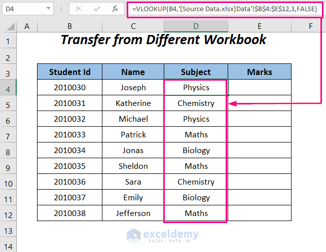
=VLOOKUP(B4,'C:\Users\Mima\Downloads\[Source Data.xlsx]Data'!$B$4:$E$12,4,FALSE)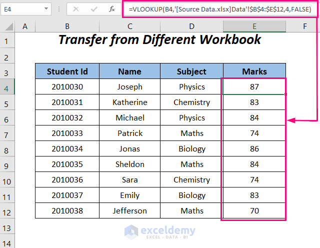
Useful Alternatives to Transfer Data with VLOOKUP
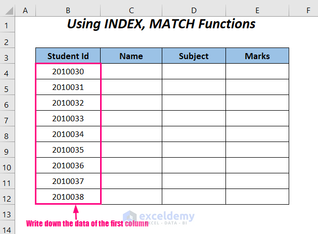
Method 1 – Using INDEX-MATCH Formula to Transfer Data from One Excel Worksheet to Another
Steps:
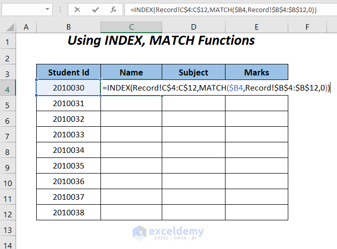
Write down the data of the first column, Student ID, first.
➤ Type the following formula in cell C4.
=INDEX(Record!C$4:C$12,MATCH($B4,Record!$B$4:$B$12,0))B4 is the lookup value, Record!$B$4:$B$12 is the lookup range of the Record sheet, and C$4:C$12 is the range containing output values.
- MATCH($B4,Record!$B$4:$B$12,0) becomes
MATCH(2010030, Record!$B$4:$B$12,0) → MATCH will give the row index number of the value 2010030 in the range $B$4:$B$12 of the Record sheet.
Output → 1
- INDEX(Record!C$4:C$12,MATCH($B4,Record!$B$4:$B$12,0)) becomes
INDEX(Record!C$4:C$12,1,0)) → returns the name of the student for the ID 2010030
Output → Joseph
➤ Press ENTER.
➤ Drag the Fill Handle tool to the right and down.
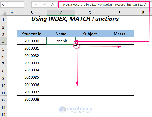
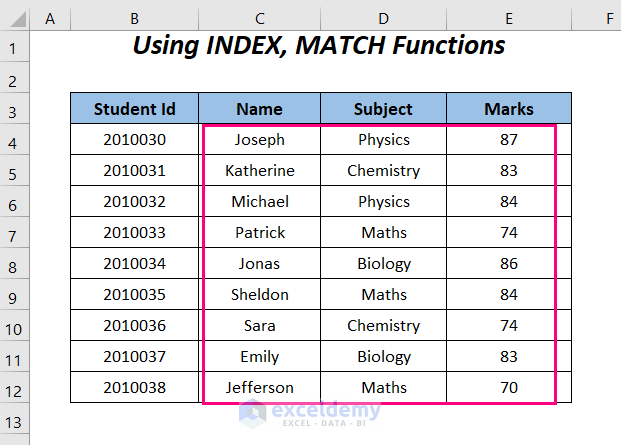
You will have all the data from the source sheet on this sheet.
Method 2 – Using INDIRECT, ADDRESS, ROW, and COLUMN Functions to Transfer Data from One Worksheet to Another
Steps:
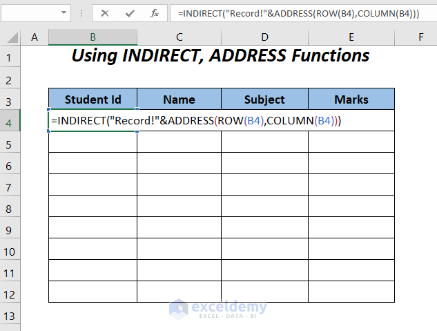
Apply the following formula in cell B4.
=INDIRECT("Record!"&ADDRESS(ROW(B4),COLUMN(B4)))- ROW(B4) → returns the row number of the cell B4
Output → 4
- COLUMN(B4) → returns the column number of the cell B4
Output → 2
- ADDRESS(ROW(B4),COLUMN(B4)) becomes
ADDRESS(4,2) → returns the reference of a cell with Row 4 and Column 4.
Output → $B$4
- INDIRECT(“Record!”&ADDRESS(ROW(B4),COLUMN(B4))) becomes
INDIRECT(“Record!”&$B$4) → INDIRECT(“Record!$B$4”)
Output → 2010030
➤ Press ENTER.
➤ Drag the Fill Handle tool to the right and down.
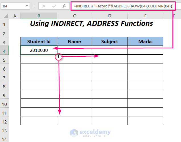
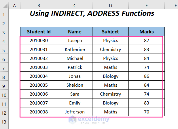
Move all of the data from our source datasheet to this sheet.
Download Workbook
Related Articles
- 10 Best Practices with VLOOKUP in Excel
- 7 Practical Examples of VLOOKUP Function in Excel
- VLOOKUP Example Between Two Sheets in Excel
- How to Use Dynamic VLOOKUP in Excel
- How to Make VLOOKUP Case Sensitive in Excel
- VLOOKUP from Another Sheet in Excel
- How to Use VLOOKUP Formula in Excel with Multiple Sheets
- How to Remove Vlookup Formula in Excel
- How to Apply VLOOKUP to Return Blank Instead of 0 or NA
- How to Hide VLOOKUP Source Data in Excel
- How to Copy VLOOKUP Formula in Excel
<< Go Back to VLOOKUP Between Worksheets | Excel VLOOKUP Function | Excel Functions | Learn Excel
Get FREE Advanced Excel Exercises with Solutions!

for Methods 1-4 you should peg cell address to column B
as-is
=VLOOKUP(B4,Record!B4:E12,2,FALSE)
to-be
=VLOOKUP($B4,Record!B4:E12,2,FALSE)
interestingly in the Alternatives Method 1 you do agree, specifying
=INDEX(Record!C$4:C$12,MATCH($B4,Record!$B$4:$B$12,0))
Hello Dick Baker,
Thank you for your insightful feedback! Pegging the column reference in the VLOOKUP formula using $B4 ensures more consistent results when copying the formula across columns. We appreciate you pointing this out, and it’s great to see your attention to detail!
As you noticed, we did apply absolute references correctly in the alternative method using INDEX and MATCH. We’ll make sure to update the earlier examples for consistency and clarity.
Thanks again for helping us improve the content!
Regards
ExcelDemy
the standard Excel library contains functions IFERROR(), IFNA() which provide the 2nd [mandatory] parameter (value_if_error or value_if_na).
It is significant that MS do not provide an equivalent IFBLANK() function to satisfy this common requirement, instead of the STUPID scenarios of having to invoke the [expensive] VLOOKUP() function twice.
MS should be STRONGLY urged to implement this long-overdue functionality !
Hello Dick Baker,
Thank you for your comment and for sharing your perspective!
You’re absolutely right, while IFERROR() and IFNA() are incredibly useful for handling error scenarios, the absence of a built-in IFBLANK() function does leave a noticeable gap for handling blank cells more efficiently. As you mentioned, having to call functions like VLOOKUP() twice just to manage blanks is not optimal, especially for larger datasets where performance matters.
We agree that a native IFBLANK() function would simplify formulas and improve usability. Your suggestion is valid, and we hope Microsoft considers incorporating such a feature in future Excel updates.
Thanks again for your thoughtful input, it adds great value to the discussion!
Regards
ExcelDemy