When you have to deal with massive data from multiple worksheets across your Excel workbook, the VLOOKUP function is your savior. The VLOOKUP function is one of the most useful and at the same time one of the most sophisticated functions in Excel. This function helps you to assemble your data from multiple data sheets in an organized way. Today, in this article we will discuss how to use the VLOOKUP function from another sheet in Excel.
Overview of VLOOKUP Function in Excel
In plain language, the VLOOKUP function takes the user’s input, looks up it in the Excel worksheet, and returns an equivalent value related to the same input. This function is available in all versions of Excel from Excel 2007.
- Summary
The VLOOKUP function takes the input value, searches it in the worksheets, and returns the value matching the input.
- Syntax
- Argument
| Argument | Required/Optional | Explanation |
|---|---|---|
| lookup_value | Required | The value we want to find by searching it in another worksheet |
| table_array | Required | The range of cells in another worksheet containing out input data |
| col_index_num | Required | The specific column number in the sheet_range containing the information we want to achieve |
| [range_lookup] | Optional | The value is either TRUE or FALSE. False for an exact match and TRUE for an appropriate match. |
- Output
Returns an exact or approximate value equivalent to the user’s input value.
VLOOKUP from Another Sheet: 2 Cases
You may need to apply the VLOOKUP function to look up values either from a different single worksheet or multiple worksheets. Let’s demonstrate these two different Cases.
1. VLOOKUP from Another Single Sheet
In this type, we will learn how to use the VLOOKUP function when you have to retrieve data from another sheet in the same workbook.
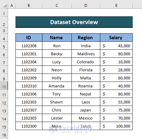
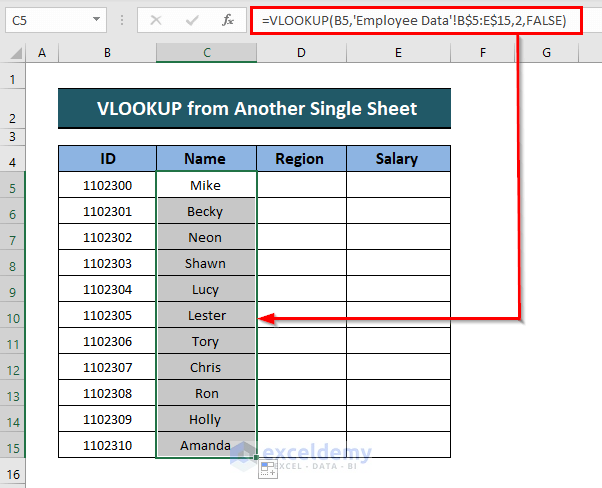
Consider a dataset where the “ID” number, Sales Rep’s “Name”, “Region” and “Salary” is given like the given one in the image. In this dataset, the ID numbers are given arbitrarily. Our task is to put the ID number in another worksheet and retrieve the information related to the ID number.
🔗 Steps:
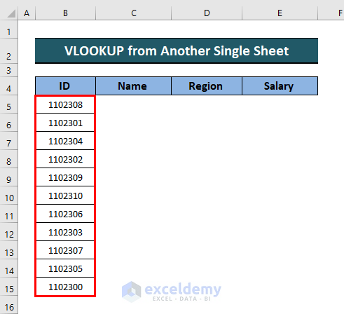
- First of all, create another worksheet where we want to get the information matching the ID number using the VLOOKUP function.
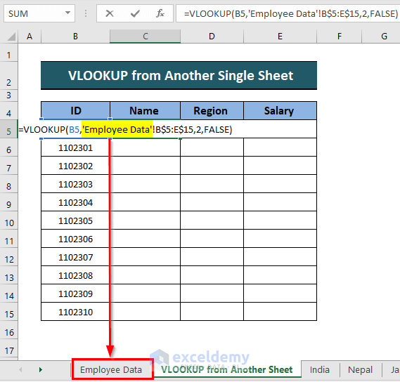
- Then, apply the VLOOKUP function in the Name Column,
=VLOOKUP(B5,'Employee Data'!B$5:E$15,2,FALSE)
Here,
- Lookup_value is B$5
- table_array: is ‘Employee Data’!B$4:E$14 (Click on the employee data worksheet and select the array)
- Col_index_num is 2
- [range_lookup]: we want the exact match (FALSE)
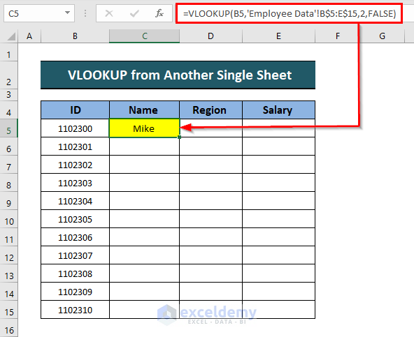
- Now, press “ENTER” to get your value from another worksheet.
- Next, select the cell that contains the function. Shift your cursor to the corner of the cell until you see this icon. That icon is called Fill Handle. Drag the tool downward to Autofill the formula to the next cells.

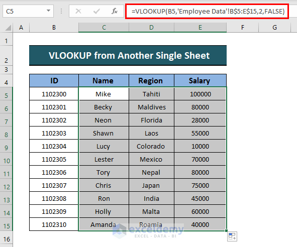
- As a result, you will get the same result for the rest of the ID numbers.
It is noticeable that we have used the lookup range as “B$4:E$14” which means we have locked the column. So with copying or dragging the formula, the cell reference won’t change itself further. If we had used Absolute cell reference (i.e. $B$4:$E$14), both the row and column would have been frozen. Read this article to copy formulas without changing cell references and this one for changing one reference only.
- After that, hold the Fill Handle with the column Name selected and drag the mouse to the right-end corner to get the rest of the result.

- Hence, all the rest of the cells will fill themselves with the VLOOKUP function.
2. VLOOKUP from Multiple Sheets
When we have to look up values between two or more multiple sheets, the previous method is not that comfortable. The best solution is to use the VLOOKUP function with nested IFERROR or Nested INDIRECT functions to look up between worksheets one by one. We will now learn it.
2.1. Using IFERROR Function
Let’s assume that we have three worksheets containing employee data from the “India”, “Nepal”, and “Japan” regions.


We want to find their salary in a new worksheet using their ID number as input with VLOOKUP nested in the IFERROR function. The format for this formula is:
If no value is found, the formula will return “NOT FOUND”.
🔗 Steps:
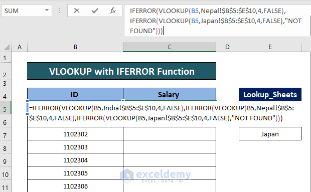
- At first, make a new worksheet containing the ID number and Salary column. In the ID column, input the ID number that you want to look up in those sheets.

- Now, apply the following formula that contains the VLOOKUP with the IFERROR function.
=IFERROR(VLOOKUP(B5,India!$B$5:$E$10,4,FALSE),IFERROR(VLOOKUP(B5,Nepal!$B$5:$E$10,4,FALSE),IFERROR(VLOOKUP(B5,Japan!$B$5:$E$10,4,FALSE),"NOT FOUND")))
Where,
- Lookup_Value is B5
- Sheet_range is India!$B$5:$E$10, Nepal!$B$5:$E$10, Japan!$B$5:$E$10
- Col_index_num is 4
- Range_lookup is False as we want an Exact Match
- Then, press ENTER so that we get our value.

- Next, copy the formula for the rest of the cells.

We can see that in ID number “1102316”, the value is “NOT FOUND”. Because this ID number does not exist in those worksheets. So, VLOOKUP from another sheet in Excel is done here.
Read More: VLOOKUP Example Between Two Sheets in Excel
2.2. Using INDIRECT Function
There is another way to VLOOKUP between multiple sheets in Excel by using a combination of the “VLOOKUP” and the “INDIRECT” functions along with INDEX, MATCH, and COUNTIF functions. We have now an extra worksheet named “Africa” along with the 3 lookup sheets stated in Method 2.1.

Now we will consider four different worksheets containing employee information to apply this formula. Create a new worksheet where we will compile that information. The format of the formula we want to use will be:
=VLOOKUP(lookup_value, INDIRECT("'"&INDEX(Lookup_sheets, MATCH(1, --(COUNTIF(INDIRECT("'" &Lookup_sheets& "'!lookup_range"), lookup_value)>0), 0)) & "'!table_array"), col_index_num, FALSE)🔗 Steps:
- We named those worksheets “India”, “Nepal”, “Japan” and “Africa”. Now write all of the lookup sheets in any cell of your workbook and name that range.

- Next, apply the following formula:
=VLOOKUP($B5,INDIRECT("'"&INDEX(Lookup_Sheets,MATCH(1,--(COUNTIF(INDIRECT("'"&Lookup_Sheets&"'!$B$5:$B$10"),$B5)>0),0))&"'!$B$5:$E$10"),4,FALSE)
Where,
- Lookup_value is $B5.
- Lookup_sheets is the named range containing the names of the sheets.
- Lookup_range is the column range to look up for ($B$5:$B$10)
- Table_array is the data range ($B$5:$E$10)
- Col_index_num is
- “FALSE” is for the exact match.

This is an array formula. So we will press SHIFT+CTRL+ENTER simultaneously to apply this formula.
💡 Formula Explanation
INDIRECT(“‘”&INDEX(Lookup_Sheets,MATCH(1,–(COUNTIF(INDIRECT(“‘”&Lookup_Sheets&”‘!$B$5:$B$10″),$B5)>0),0))&”‘!$B$5:$E$10”) => this segment is the lookup array for VLOOKUP function. Let’s explain it.
Lookup_sheets is a named range with value=> India, Nepal, Japan, Africa
INDIRECT(“‘”&Lookup_Sheets&”‘!$B$5:$B$10”) = INDIRECT{“‘India’!$B$5:$B$10″;”‘Nepal’!$B$5:$B$10″;”‘Japan’!$B$5:$B$10″;”‘Africa’!$B$5:$B$10”} => this portion returns: {1102304;1102310;1102314;1102320}
Now, (COUNTIF(INDIRECT(“‘”&Lookup_Sheets&”‘!$B$5:$B$10”),$B5) = COUNTIF{1102304;1102310;1102314;1102320} returns=> {1;0;0;0}
MATCH(1,–(COUNTIF(INDIRECT(“‘”&Lookup_Sheets&”‘!$B$5:$B$10”),$B5)>0),0) = MATCH(1,–({1;0;0;0}>0),0) = MATCH(1,–({TRUE;FALSE;FALSE;FALSE}),0) = MATCH(1,–{TRUE;FALSE;FALSE;FALSE},0) returns=> 1
INDEX(Lookup_Sheets,MATCH(1,–(COUNTIF(INDIRECT(“‘”&Lookup_Sheets&”‘!$B$5:$B$10”),$B5)>0),0)= INDEX(Lookup_Sheets,1) returns => “India”
So, at this moment, the formula turns out to be => VLOOKUP($B5,INDIRECT(“‘”&”India”&”‘!$B$5:$E$10”),4,FALSE)
INDIRECT(“‘”&”India”&”‘!$B$5:$E$10”) returns the array $B$5:$E$10 from the sheet India => {1102304,”Ronand”,”India”,44000;1102302,”Duke”,”India”,56000;1102303,”Lucy “,”India”,98000;1102301,”Neon “,”India”,23000;1102300,”Hector”,”India”,12000;1102305,”Holly “,”India”,56000}
So, the final Output is=> $12000
We got our value matching the same ID number. Now apply the same formula for the rest of the ID. If there is any non-existing ID, The return value is “#N/A”.
Things to Remember
➤ The VLOOKUP function always searches for lookup values from the leftmost top column to the right. This function “Never” searches for the data on the left.
➤ If you enter a value less than “1” as the column index number, the function will return an error.
➤ When you select your “Table_Array” you have to use the absolute cell references ($) to block the array.
➤ Since the combination of the VLOOKUP and the INDIRECT function is an “Array formula” you have to press SHIFT+CTRL+ENTER to apply the formula.
Download Practice Workbook
Download this practice sheet to practice while you are reading this article.
Conclusion
Searching for data in one or multiple worksheets and compiling them systematically with the VLOOKUP function from another sheet is discussed in this article. Though this function is difficult for the new users to comprehend, we tried to make it as simple as possible. Hope this article is useful for you. Share your thoughts if you have any confusion.
Related Articles
- 10 Best Practices with VLOOKUP in Excel
- 7 Practical Examples of VLOOKUP Function in Excel
- How to Use Dynamic VLOOKUP in Excel
- Transfer Data from One Excel Worksheet to Another Automatically with VLOOKUP
- How to Make VLOOKUP Case Sensitive in Excel
- How to Remove Vlookup Formula in Excel
- How to Apply VLOOKUP to Return Blank Instead of 0 or NA
- How to Hide VLOOKUP Source Data in Excel
- How to Copy VLOOKUP Formula in Excel
<< Go Back to VLOOKUP Between Worksheets | Excel VLOOKUP Function | Excel Functions | Learn Excel
Get FREE Advanced Excel Exercises with Solutions!

Hi Asikul Islam,
I am delighted to see your wonderful development of exceldemy website focusing on the detail learning on microsoft excel. It’s really amazing to have an advanced knowledge on microsoft excel from your exceldemy website. I passed my graduation and post graduation from BUET. Presently, I am giving my attention and interest on data analysis and data science. I hope, your exceldemy will help me to learn more advanced functions in my journey to data analysis / data science. I wish you success in your further development and more creativity.
– Nasir Ahmed, Dhaka
Hello Nasir Ahmed,
Thanks for your appreciation.
Regards
ExcelDemy