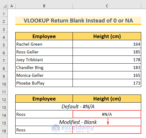
We will use a dataset with two columns, “Employee” and “Height(cm),” to demonstrate our methods. The value “Ross” is not listed on the primary dataset. When we try to use the VLOOKUP function for that value, we get the “N/A” error in cell C14. However, we will modify the formula to show blank values instead of that error in cell C16.
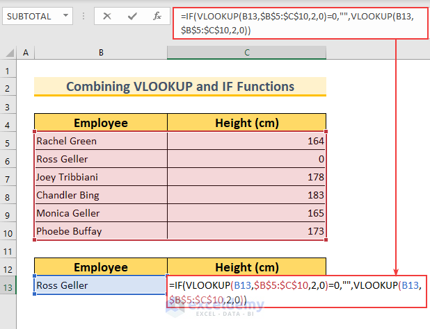
Method 1 – Combining IF and VLOOKUP Functions to Return Blank
Steps:
- Use the following formula in cell C13.
=IF(VLOOKUP(B13,$B$5:$C$10,2,0)=0,"",VLOOKUP(B13,$B$5:$C$10,2,0))
If we did not add the IF function, this function would have returned zero.
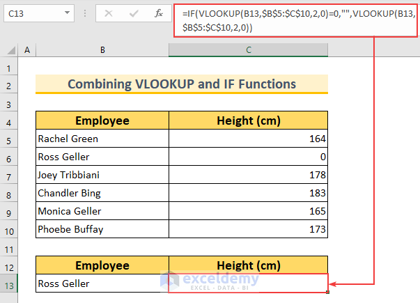
- Press Enter.
Formula Breakdown
- This formula has two identical VLOOKUP functions. The first one has a condition attached to it that checks if it equals 0. If it is not, then the second VLOOKUP function executes.
- VLOOKUP(B13,$B$5:$C$10,2,0)
- Output: 0.
- This function looks for the value from cell B13 in the range of B5:C10. If there is a match, then it returns the value from the respective C5:C10 range as indicated by 2 inside the function. The 0 means at the end of this function the match type is exact.
- Our formula reduces to → IF(0=0,””,0)
- Output: (Blank).
- Here the logical_test is true, so we have the blank output.
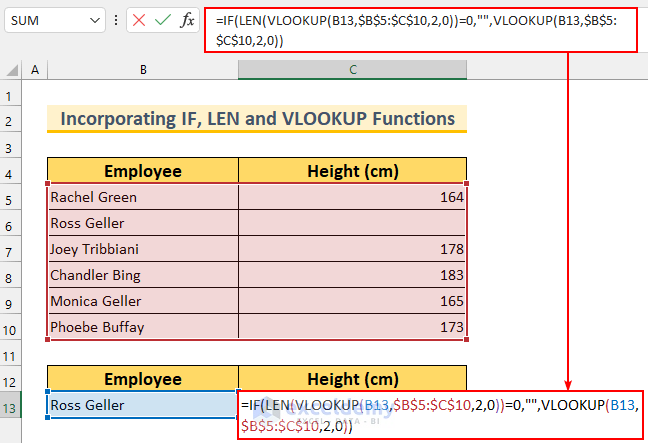
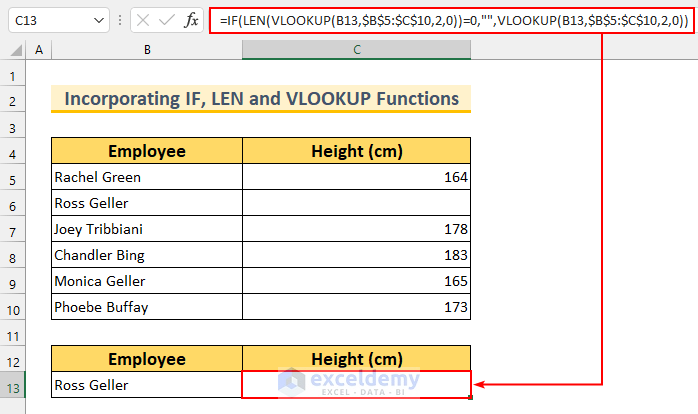
Method 2 – Incorporating IF, LEN, and VLOOKUP Functions to Return Blank
Steps:
- Use the following formula in cell C13.
=IF(LEN(VLOOKUP(B13,$B$5:$C$10,2,0))=0,"",VLOOKUP(B13,$B$5:$C$10,2,0))
- Hit Enter.
Formula Breakdown
- This formula has two VLOOKUP functions. Moreover, we have used the first VLOOKUP function inside a LEN function, which returns the length of a string. Now, the length of a blank cell is 0. So, we have set this in the logical_test criteria.
- VLOOKUP(B13,$B$5:$C$10,2,0)
- Output: 0.
- This function looks for the value from cell B13 in the range of B5:C10. If there is a match, then it returns the value from the respective C5:C10 range as indicated by 2 inside the function. The 0 means at the end of this function the match type is exact.
- Our formula reduces to → IF(LEN(0)=0,””,0)
- Output: (Blank).
- The LEN function returns 0. So, the first portion of the IF function executes and we get the blank cell as the output.
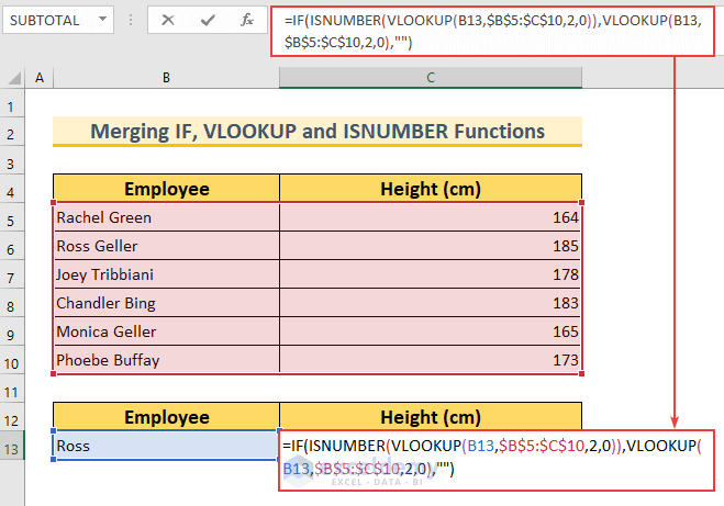
Method 3 – Merging IF, ISNUMBER, and VLOOKUP Functions to Return Blank
Steps:
- Use the following formula in cell C13.
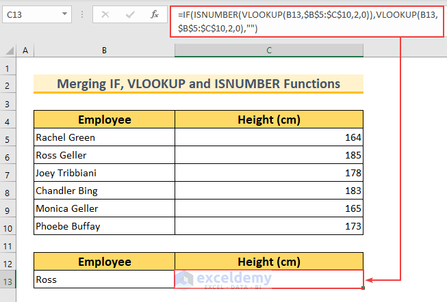
=IF(ISNUMBER(VLOOKUP(B13,$B$5:$C$10,2,0)),VLOOKUP(B13,$B$5:$C$10,2,0),"")
- Press Enter.
Formula Breakdown
- This formula has two VLOOKUP functions. We have used the first VLOOKUP function inside an ISNUMBER function, which returns true for a number and false for a non-numerical output. Now, if the first VLOOKUP function returns an error, then it will not be a number. So, we have set this in the logical_test criteria, and when that happens the false portion of the IF function will execute.
- VLOOKUP(B13,$B$5:$C$10,2,0)
- Output: #N/A.
- This function looks for the value from cell B13 in the range of B5:C10. If there is a match, then it returns the value from the respective C5:C10 range as indicated by 2 inside the function. Moreover, the value “Ross” cannot be found in the specified cell range, hence it has shown the error. The 0 means at the end of this function the match type is exact.
- Our formula reduces to → IF(ISNUMBER(#N/A),#N/A,””)
- Output: (Blank).
- The ISNUMBER function returns 0, which means false. So, the second portion of the IF function executes and we get the blank cell as the output.
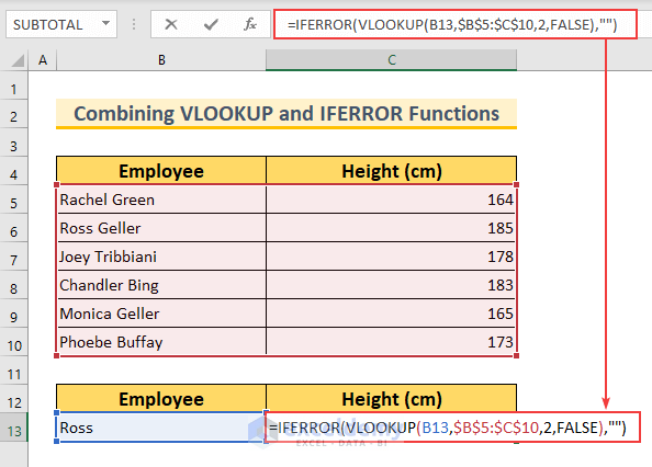
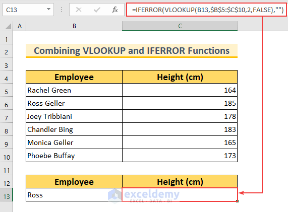
Method 4 – Combining IFERROR and VLOOKUP Functions
Steps:
- Use the following formula in cell C13.
=IFERROR(VLOOKUP(B13,$B$5:$C$10,2,FALSE),"")
- Hit Enter.
Formula Breakdown
- This formula has a single VLOOKUP function, and we have used this inside an IFERROR function, which returns modified output in the case of an error. Now, the modified output is set to a blank cell.
- VLOOKUP(B13,$B$5:$C$10,2,FALSE)
- Output: 0.
- This function looks for the value from cell B13 in the range of B5:C10. If there is a match, then it returns the value from the respective C5:C10 range as indicated by 2 inside the function. The FALSE at the end of this function means the match type is exact.
- Our formula reduces to → IFERROR(#N/A,””)
- Output: (Blank).
- This function modifies any errors and returns the blank cell as the output.
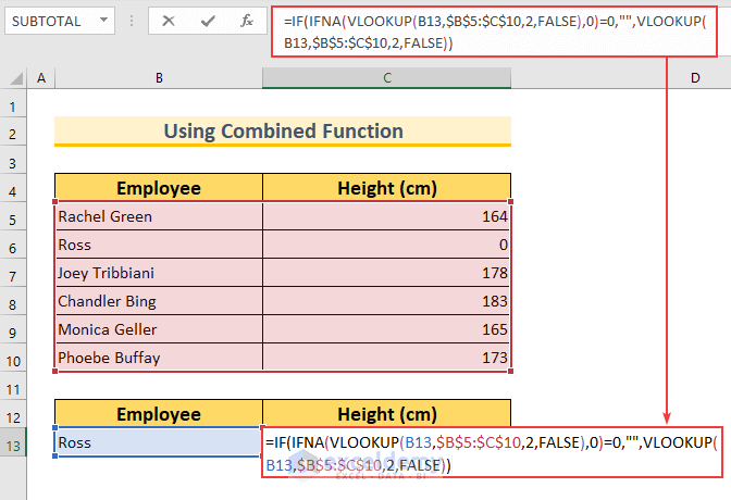
Method 5 – Using Combined Functions to Return Blank Instead of 0 or #N/A! Error
Steps:
- Use the following formula in cell C13.
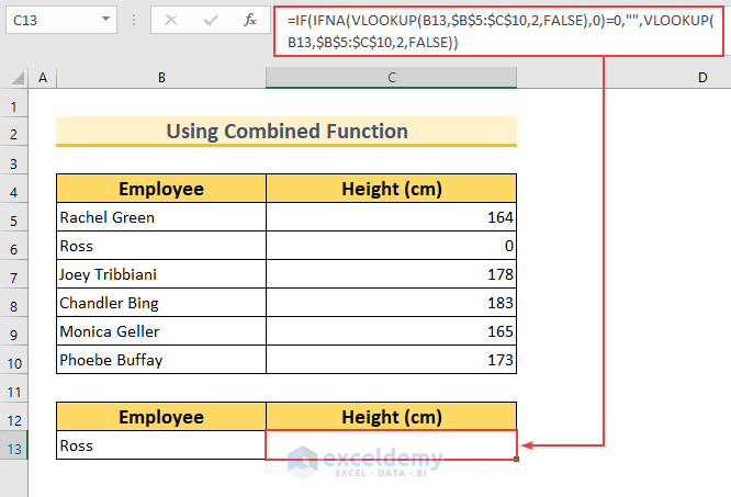
=IF(IFNA(VLOOKUP(B13,$B$5:$C$10,2,FALSE),0)=0,"",VLOOKUP(B13,$B$5:$C$10,2,FALSE))
- Press Enter.
Formula Breakdown
- This formula has two VLOOKUP functions. Moreover, we have used the first VLOOKUP function inside an IFNA function, which checks for the “#N/A” error. If it finds the error, then it will return 0. Otherwise, it will return the original output. We have set it so that when it finds 0, it will return a blank cell.
- Now, VLOOKUP(B13,$B$5:$C$10,2,FALSE)
- Output: 0.
- This function looks for the value from cell B13 in the range of B5:C10. If there is a match, then it returns the value from the respective C5:C10 range as indicated by 2 inside the function. The FALSE at the end of this function means the match type is exact.
- Our formula reduces to → IF(IFNA(0,0)=0,””,0)
- Output: (Blank).
- The IFNA function returns 0, which means the logical_test is true. So, the first portion of the IF function executes and we get the blank cell as the output.
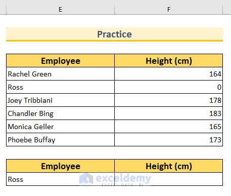
Practice Section
We have added a practice dataset for each method in the Excel file.
Download the Practice Workbook
Related Articles
- 10 Best Practices with VLOOKUP in Excel
- 7 Practical Examples of VLOOKUP Function in Excel
- VLOOKUP Example Between Two Sheets in Excel
- How to Use Dynamic VLOOKUP in Excel
- Transfer Data from One Excel Worksheet to Another Automatically with VLOOKUP
- How to Make VLOOKUP Case Sensitive in Excel
- VLOOKUP from Another Sheet in Excel
- How to Use VLOOKUP Formula in Excel with Multiple Sheets
- How to Remove Vlookup Formula in Excel
- How to Hide VLOOKUP Source Data in Excel
- How to Copy VLOOKUP Formula in Excel
<< Go Back to Issues with VLOOKUP | Excel VLOOKUP Function | Excel Functions | Learn Excel
Get FREE Advanced Excel Exercises with Solutions!
