Issues with the VLOOKUP Function – 10 Solutions

This is an overview:

Download Practice Workbook

Download the practice workbook.

Solution 1 – The Lookup Value Is Not Found in the First Cell

There is an error due to the wrong column placement. The lookup column should be in the first position.

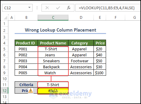
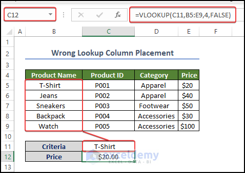
• Place the column in the first position in the lookup range.

The price is displayed in C12.

Solution 2 – Data is Missing or Not Found

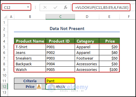
The criteria are not available in B5:B9.

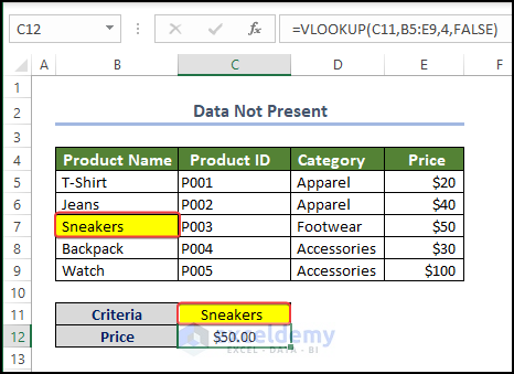
• Change the criteria to “Sneakers”.

You can see the price in C12.

Read More: Why VLOOKUP Returns #N/A When Match Exists 

Solution 3 – Format Mismatch (Apostrophe Saved As Text)

There is an apostrophe before the text. B5:B9 is formatted as text.

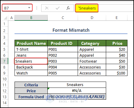
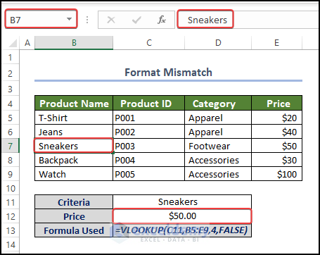
• Remove the apostrophe.

You can see the price in C12.

Read More: VLOOKUP Not Working Due to Format

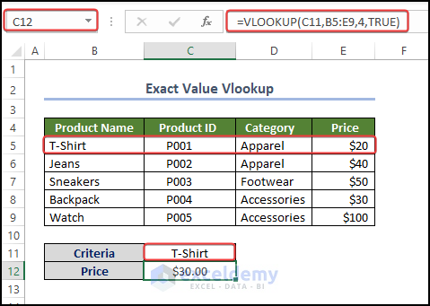
Solution 4 – Exact Match Vs Approximate Match

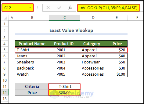
In the VLOOKUP function, the last argument refers to an exact match (False) or an approximate match (True). If False is used and there isn’t an exact match, the output will be N/A.

• TRUE was used as an argument in the formula. The output is an approximate value:

• If the FALSE argument is used, the correct price is displayed:

Solution 5 – Locked Table Reference

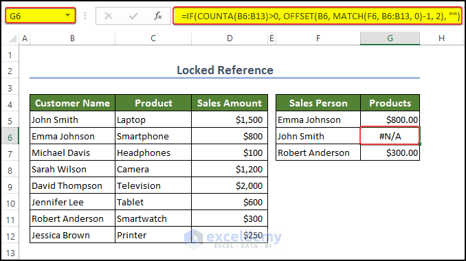
In the formula in G5, the reference to the lookup range is locked.

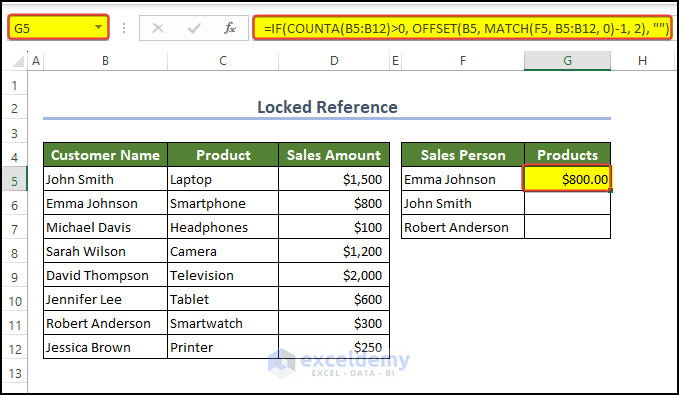
If you drag the Fill Handle to G7, you get incorrect values.

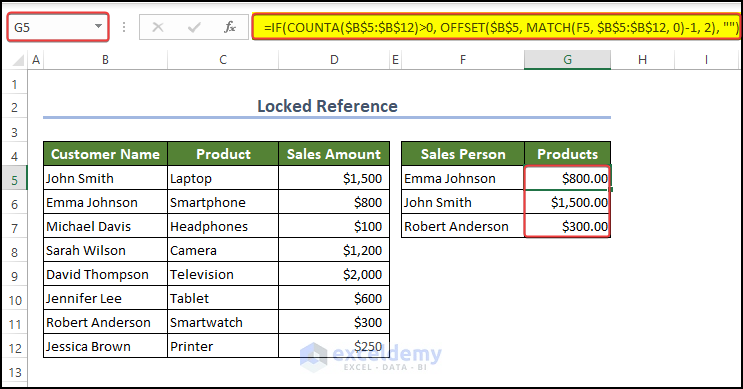
• Enter the modified formula in G5.

• Drag the Fill Handle to G7.

 The correct values are displayed.

Solution 6 –Duplicate Values

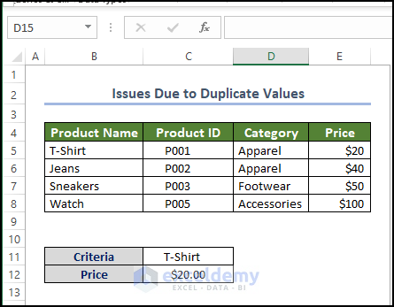
In the below image, there are duplicate values in B5:E9, causing an incorrect output in C12. 

• Select B5:E9.
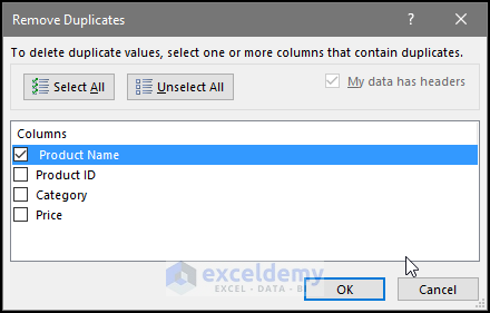
• Go to Data > Data Tools > Remove Duplicates.

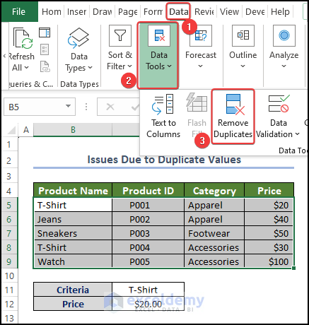
• In Remove Duplicates, check the column containing duplicates.
• Click OK.

Duplicate values are removed and the correct price is displayed.

Solution 7 –Wrong Index Number

If the index number is wrong or less than 1, an error is displayed in C12.

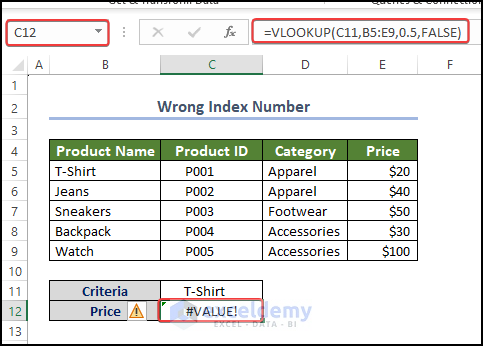
The index number in the formula is less than 1.

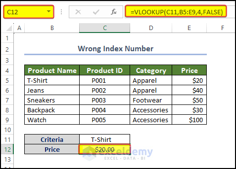
• Correct it to 4.

Solution 8 – Showing the Formula As Text

The formula is displayed in the cell, but not the output.

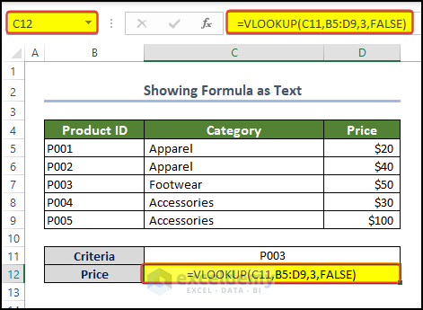
The cell is in text format.

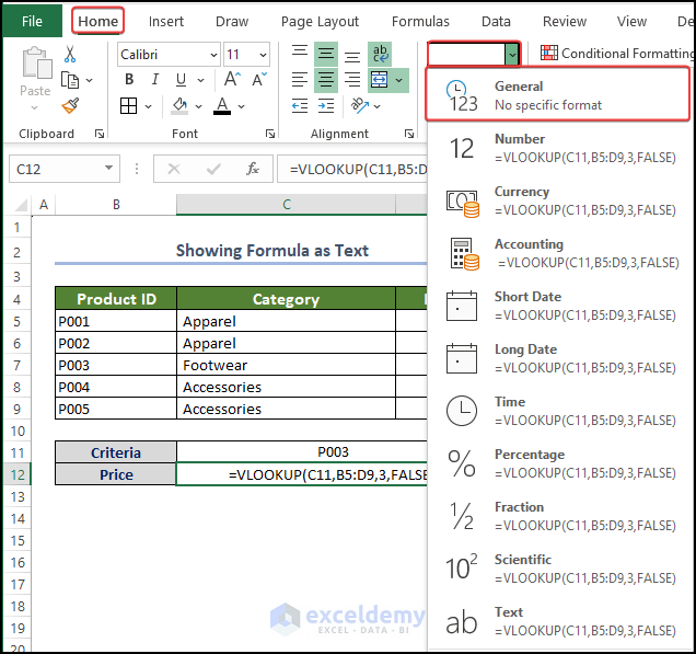
• Select the cell and go to Home > Number.
• Change the cell format to General.
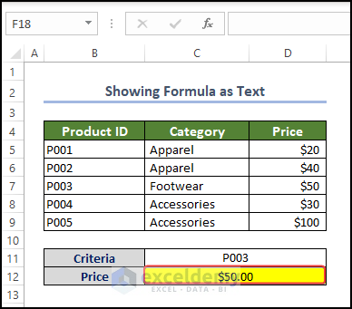
• Re-enter the formula.

The output is displayed.

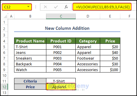
Solution 9 – Adding New Columns 

There is a VLOOKUP formula in C12  and the output is correctly displayed.

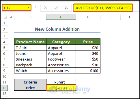
A new column is added between columns B and D. The formula returns other values.

In the formula, the third column was declared as the return column.

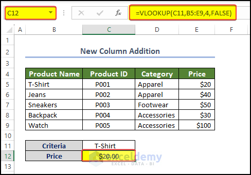
• Change the formula and enter it into the cell.

Read More: Excel VLOOKUP Drag Down Not Working

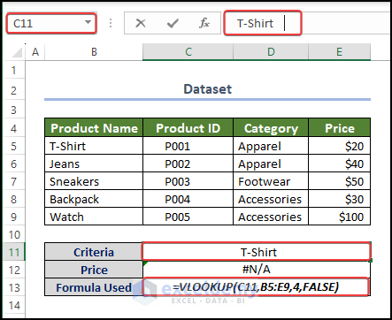
Solution 10 – Hidden Space

There is an error due to a space after T-Shirt.

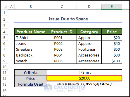
After removing the space, the price is correctly displayed.

Things to Remember

Check the column index number:  Specify the correct column index number as “col_index_num” argument. It represents the column in the data range and starts with 1 from the leftmost column.

Consider sorting data: Sort data in ascending order. Use “TRUE” for approximate matches when working with unsorted data.

Handle errors with IFERROR: Wrap your VLOOKUP formula within the IFERROR function. This allows you to specify an alternative result or an error message when no match is found.

Use absolute cell references: When copying the VLOOKUP formula to other cells, ensure the cell references are absolute (e.g., $A$1) for the lookup range and relative (e.g., A1) for the lookup value.

Frequently Asked Questions

Q1. What are the disadvantages of VLOOKUP?

It has limited search capabilities, requires an exact match, is inefficient with large datasets, can’t handle multiple matches, and is not flexible.

Q2. What function can I use instead of VLOOKUP?

Use the INDEX-MATCH and the XLOOKUP.

The INDEX-MATCH combines the INDEX and MATCH functions. Instead of searching for a value in a single column, the MATCH function finds the position of the value in a specified column. The INDEX function returns the corresponding value from another column based on the position returned by the MATCH function.

The XLOOKUP function allows you to search for a value in a table and return information from any column. It can handle approximate matches, array inputs, and multiple criteria.

Issues with VLOOKUP: Knowledge Hub

<< Go Back to Excel VLOOKUP Function | Excel Functions | Learn Excel