Here’s an overview of using the INDEX-MATCH and the VLOOKUP functions in a dataset.
INDEX-MATCH vs. VLOOKUP Function in Excel: 9 Examples
To show the differences between the INDEX-MATCH formula and the VLOOKUP function, we are using two tables here.
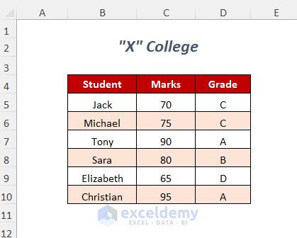
One is the Student records of a college.
Another table contains different Item records of a company.

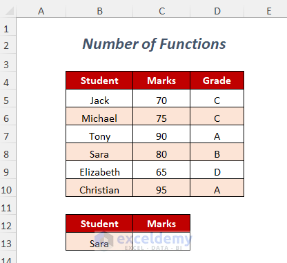
Example 1 – Number of Functions
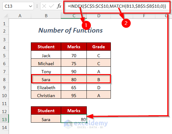
We will look up the Marks of a Student Sara by using both the INDEX-MATCH function and the VLOOKUP function.
INDEX-MATCH Function:
=INDEX($C$5:$C$10,MATCH(B13,$B$5:$B$10,0))So, here we can see this formula consists of two functions one is the INDEX function and the other is the MATCH function. Inside the MATCH function here B13 is the lookup value, $B$5:$B$10 is the lookup array and 0 is for an exact match. Finally, MATCH will return the row or column index number of the lookup value in the data range.
MATCH will return here 4.
Then, it will pass this information to the INDEX function which returns the information we actually want by using the return range $C$5:$C$10.
VLOOKUP Function:
=VLOOKUP(B13,$B$5:$D$10,2, FALSE)This formula consists of only one function which is the VLOOKUP function.
Here, B13 is the lookup value, $B$5:$D$10 is the table array, 2 is the column index number and FALSE is for an exact match.

Quick Note:
Considering the above two formulas, we can say that it is easier to use the VLOOKUP function than the INDEX-MATCH function.
Read More: How to Use VLOOKUP Function with Exact Match in Excel
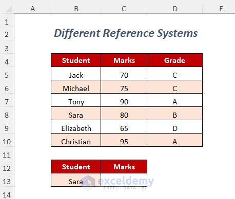
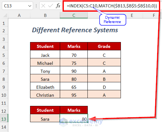
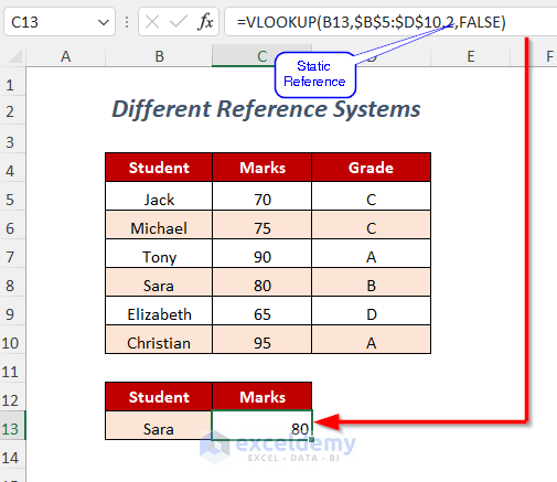
Example 2 – Different Reference Systems
We used the following table to look up the Marks for the Student Sara.
INDEX-MATCH Function:
=INDEX(C5:C10,MATCH($B13,$B$5:$B$10,0))Here, the return range C5:C10 within the INDEX function uses dynamic references so it can change with the change of the data range and give us the right output.
VLOOKUP Function:
=VLOOKUP(B13,$B$5:$D$10,2, FALSE)Here, 2 is the column index number which is the static reference in the VLOOKUP function so it cannot give us the correct value with the change of the dataset.
Quick Note:
Considering the above two formulas, we can say that it is more advantageous to use the INDEX-MATCH function than the VLOOKUP function due to the dynamic referencing.
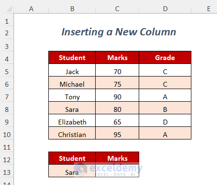
Example 3 – Inserting a New Column
We will demonstrate the changes in results after inserting a new column named Subject before the column Marks.
INDEX-MATCH Function:
=INDEX(C5:C10,MATCH($B13,$B$5:$B$10,0))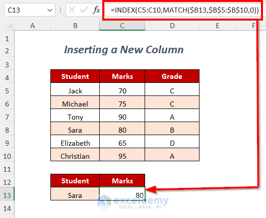
This formula is giving us the right output due to the dynamic references inside the INDEX function. It automatically changes the return range here from C5:C10 to D5:D10.
=INDEX(D5:D10,MATCH($B13,$B$5:$B$10,0))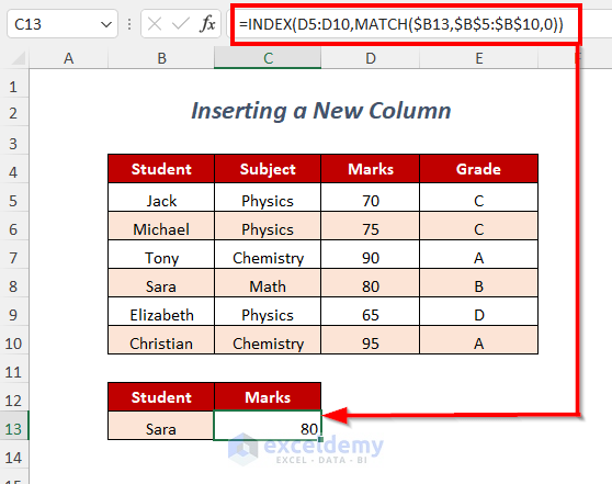
VLOOKUP Function:
=VLOOKUP(B13,$B$5:$D$10,2, FALSE)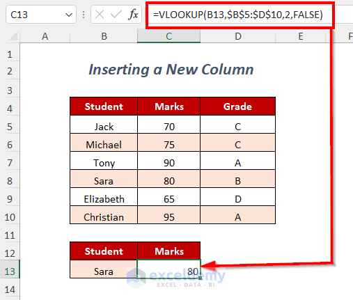
The static reference 2 doesn’t change and here the Subject column has the column index number 2.
=VLOOKUP(B13,$B$5:$E$10,2,FALSE)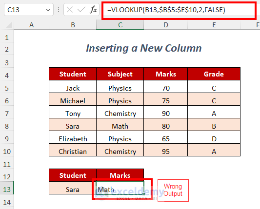
Quick Note:
Considering the above two formulas, we can say that it is more convenient to use the INDEX-MATCH function than the VLOOKUP function due to the advantages of having the correct output in spite of inserting a new column.
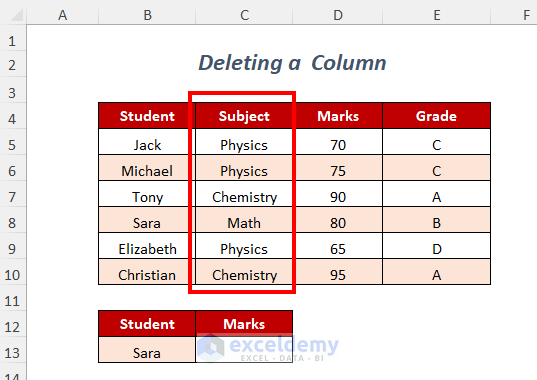
Example 4 – Deleting a Column
We will show the changes of results after deleting a column named Subject.
INDEX-MATCH Function:
=INDEX(D5:D10,MATCH($B13,$B$5:$B$10,0))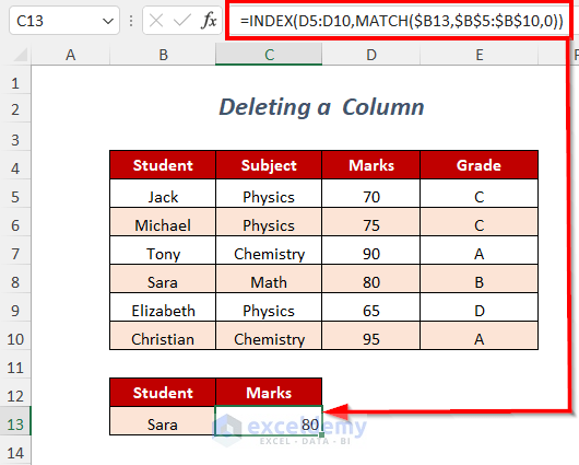
We deleted the column Subject.
This formula is giving us the right output due to the dynamic references inside the INDEX function. It automatically changes the return range here from D5:D10 to C5:C10.
=INDEX(C5:C10,MATCH($B13,$B$5:$B$10,0))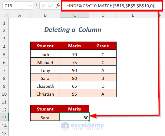
VLOOKUP Function:
=VLOOKUP(B13,$B$5:$E$10,3, FALSE)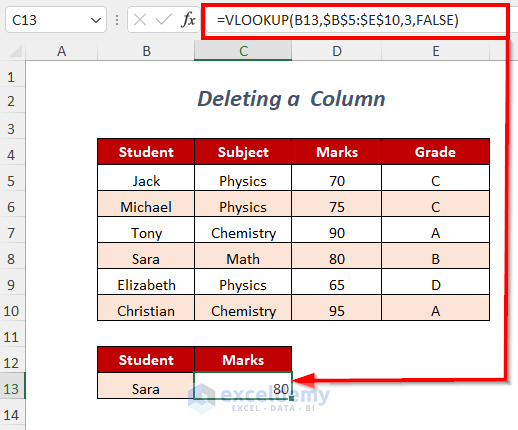
After deleting the column Subject, we are getting B instead of 80. This change occurs because static reference 3 doesn’t change and here the Grade column has the column index number 3 now.
=VLOOKUP(B13,$B$5:$D$10,3, FALSE)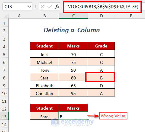
Quick Note:
Considering the above two cases, we can say that it is more convenient to use the INDEX-MATCH function than the VLOOKUP function due to the advantages of having the correct output in spite of deleting a column.
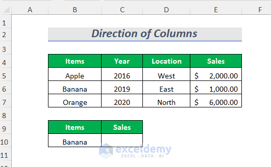
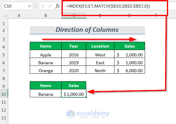
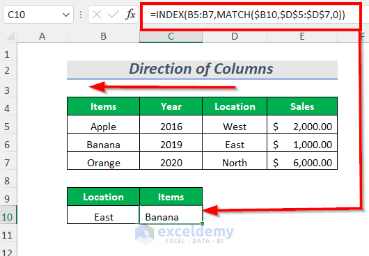
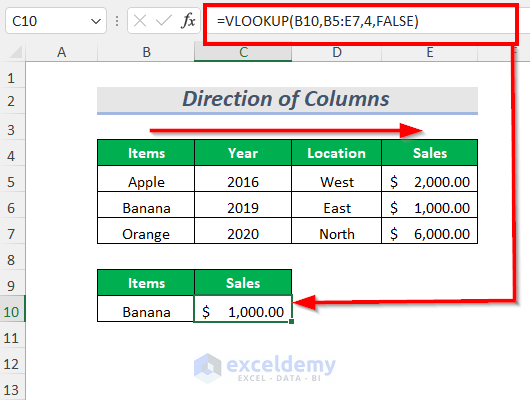
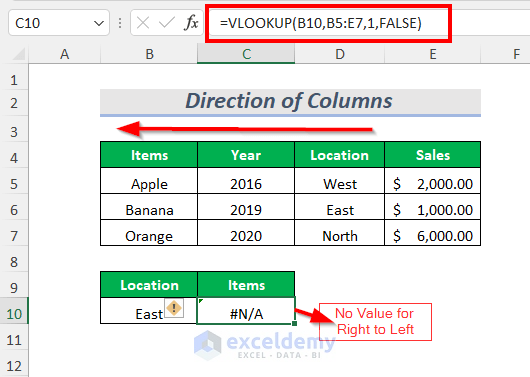
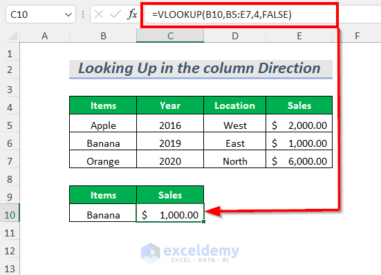
Example 5 – Direction of Columns in Range
We will show the difference in the direction of columns.
INDEX-MATCH Function:
=INDEX(E5:E7,MATCH($B10,$B$5:$B$7,0))The position of the lookup range $B$5:$B$7 is before the return range E5:E7.
=INDEX(B5:B7,MATCH($B10,$D$5:$D$7,0))The lookup range $D$5:$D$7 is after the return range B5:B7.
VLOOKUP Function:
=VLOOKUP(B10,B5:E7,4,FALSE)The position of the lookup value is in the range B5:E7 and the column index number is 4 which is after the lookup range.
=VLOOKUP(B10,B5:E7,1,FALSE)Going from the right side to the left side or having a lookup value after the return range will give us an error in this case.
Quick Note:
It is more convenient to use the INDEX-MATCH function than the VLOOKUP function due to the advantages of having the correct output regardless of the direction of the lookup range and return range.
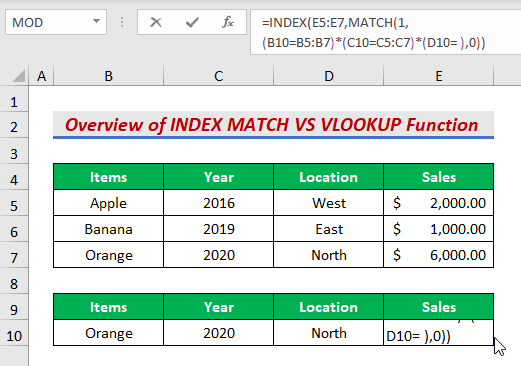
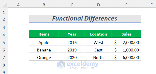
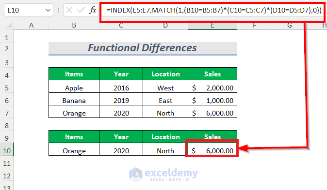
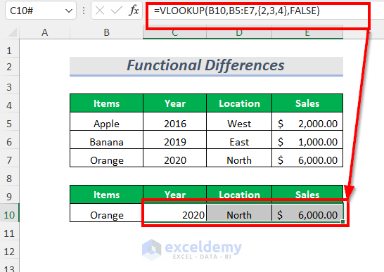
Example 6 – Functional Differences
The INDEX-MATCH function can give an output for multiple conditions whereas the VLOOKUP function can give multiple values for a lookup value.
INDEX-MATCH Function:
=INDEX(E5:E7,MATCH(1,(B10=B5:B7)*(C10=C5:C7)*(D10=D5:D7),0))B10, C10, and D10 are the lookup values that will be looked up in B5:B7, C5:C7, and D5:D7 ranges respectively and 0 is for an exact match.
MATCH will return here the row-index number 3.
Then the INDEX function will return the corresponding value.
VLOOKUP Function:
=VLOOKUP(B10,B5:E7,{2,3,4},FALSE)B10 is the lookup value, B5:E7 is the table array, {2,3,4} is the array of the column index number and FALSE is for the Exact match.
Quick Note:
The two functions can provide different results and have varied use cases.
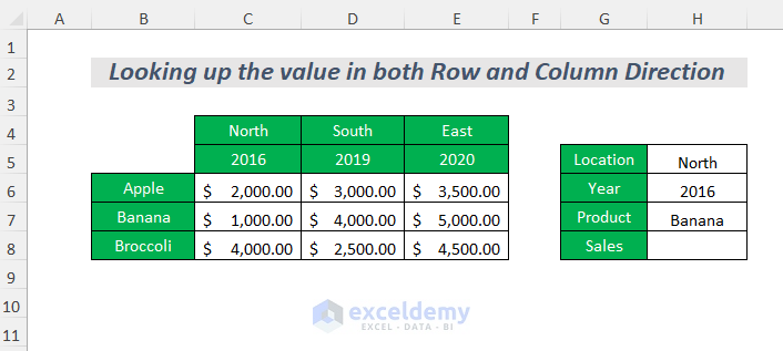
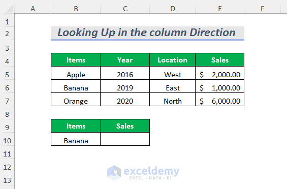
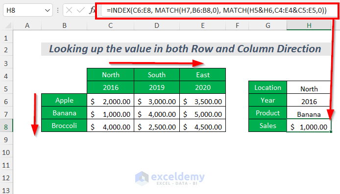
Example 7 – Looking up the Value in Row or Column or Both
The INDEX-MATCH function can look for the value in both the row-wise and column-wise direction but the VLOOKUP function can look for the value only in the column-wise direction.
INDEX-MATCH Function:
=INDEX(C6:E8, MATCH(H7,B6:B8,0), MATCH(H5&H6,C4:E4&C5:E5,0))MATCH(H7, B6:B8,0) is used for row-wise matching, and MATCH(H5&H6, C4:E4&C5:E5,0) is used for column-wise matching.
VLOOKUP Function:
=VLOOKUP(B10,B5:E7,4,FALSE)This will only look for the value in the column-wise direction.
Quick Note:
It is more convenient to use the INDEX-MATCH function than the VLOOKUP function due to the advantages of looking up the value in both the row-wise and column-wise direction rather than only the column-wise direction.
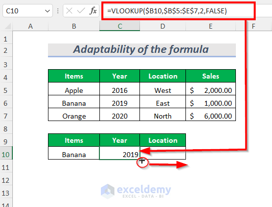
Example 8 – Adaptability of the Formula
You can easily copy or drag the formula to get the correct result in the case of the INDEX-MATCH function, but the VLOOKUP function will not give the correct result.
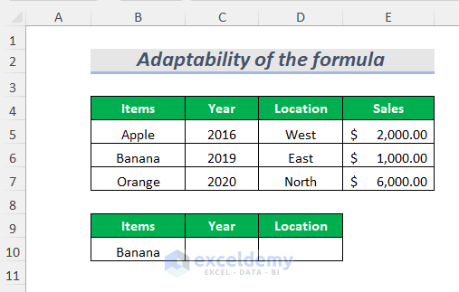
INDEX-MATCH Function:
=INDEX(C5:C7,MATCH($B10,$B$5:$B$7,0))We drag the formula to the right side.
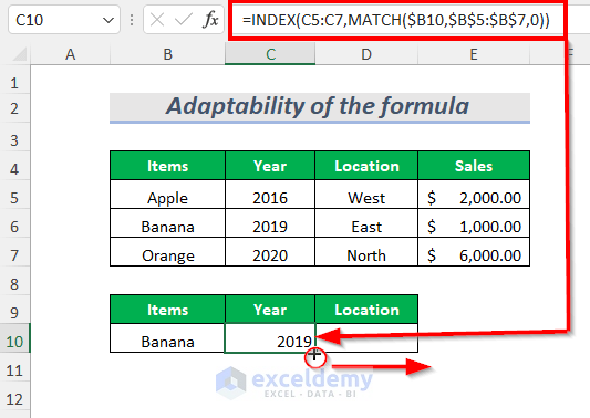
You will get the correct output East for the lookup value Banana.
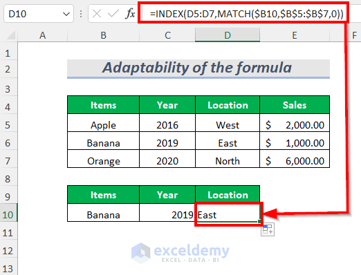
=INDEX(D5:D7,MATCH($B10,$B$5:$B$7,0))Due to the dynamic references inside the INDEX function, it automatically changes the return range here from C5:C7 to D5:D7.
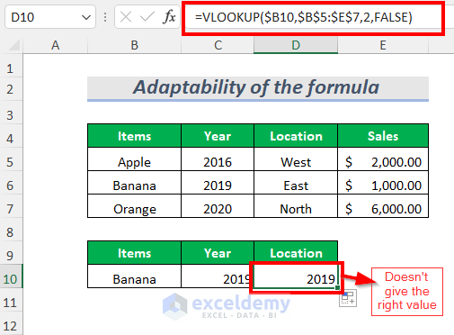
VLOOKUP Function:
We have got the Year 2019 by using the following formula
=VLOOKUP($B10,$B$5:$E$7,2,FALSE)We dragged the formula to the right.
We are not getting the correct value here.
=VLOOKUP($B10,$B$5:$E$7,2,FALSE)The formula doesn’t change here due to the static referencing, so it gives the same value as the previous one.
Quick Note:
Considering the above two formulas, we can say that it is more convenient to use the INDEX-MATCH function than the VLOOKUP function due to the advantages of having the correct output in spite of dragging or copying the formula.
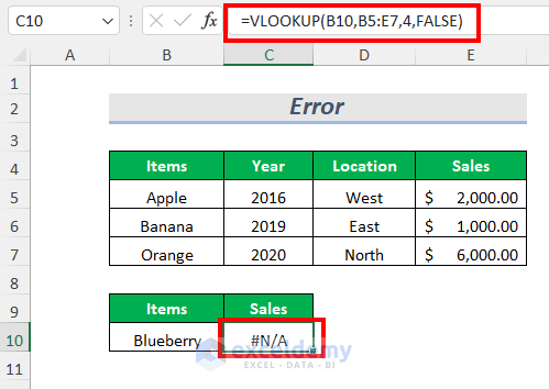
Example 9 – Errors in Formulas
In the case of the INDEX-MATCH function, you can get two errors, #REF! and #N/A, but for the VLOOKUP function only gets the #N/A error.
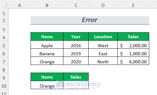
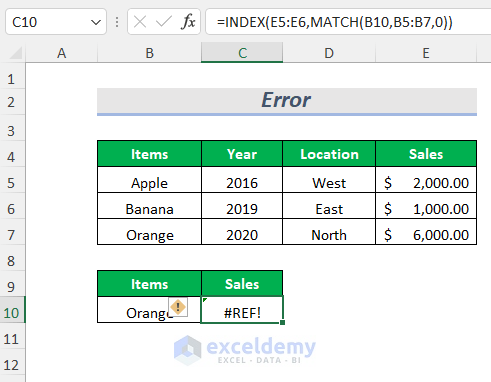
INDEX-MATCH Function:
We have mistaken the range within the MATCH function and within the INDEX function.
=INDEX(E5:E6,MATCH(B10,B5:B7,0))The selected range E5:E6 is less than the range B5:B7.
For this blunder in range selection, we are getting the #REF! error here.
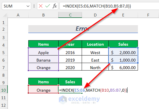
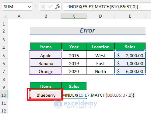
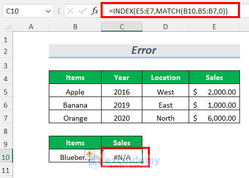
If you try to look for a value that is not in the range, you will get the #N/A error.
=INDEX(E5:E7,MATCH(B10,B5:B7,0))Blueberry is not in the range.
This will give us the #N/A error.
VLOOKUP Function:
For looking up a value that is not in the range, you will get the #N/A error.
=VLOOKUP(B10,B5:E7,4,FALSE)Blueberry is not in the range.
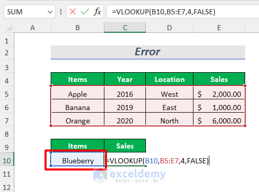
This will give us the #N/A error.
Things to Remember:
- For a look-up value exceeding 255 characters, VLOOKUP will produce an error, but the INDEX-MATCH function can work properly.
- For a large dataset, the INDEX-MATCH function is way faster than the VLOOKUP function.
- For returning multiple values, INDEX-MATCH function is better than the VLOOKUP function.
Read More: Use VLOOKUP to Sum Multiple Rows in Excel
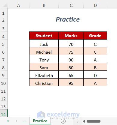
Practice Section
We have provided a Practice section like below in a sheet named Practice.
Download the Practice Workbook
Related Articles
- Combining SUMPRODUCT and VLOOKUP Functions in Excel
- How to Use VLOOKUP with COUNTIF
- How to Combine SUMIF and VLOOKUP in Excel
- Excel LOOKUP vs VLOOKUP
- XLOOKUP vs VLOOKUP in Excel
- How to Use Nested VLOOKUP in Excel
- IF and VLOOKUP Nested Function in Excel
- How to Use IF ISNA Function with VLOOKUP in Excel
- How to VLOOKUP and SUM Across Multiple Sheets in Excel
- How to Use IFERROR with VLOOKUP in Excel
- VLOOKUP with IF Condition in Excel
<< Go Back to Excel VLOOKUP Function | Excel Functions | Learn Excel
Get FREE Advanced Excel Exercises with Solutions!
