Method 1 – Using Nested VLOOKUP in Excel to Extract Product Price
Steps:
- Click on the cell that you want the Price of the ID (e.g. cell beside ID A101 in the Result Table, I5)
- Write the following formula,
=VLOOKUP(VLOOKUP(H5, $B$5:$C$9, 2, FALSE), $E$5:$F$9, 2, FALSE)Here,
H5 = A101, the ID that we stored in the Result Table as the lookup value
$B$5:$C$9 = Data range in Table 1 to search the lookup value
$E$5:$F$9 = Data range in Table 2 to search the lookup value
2 = Column index number to search the lookup value
FALSE = Want an exact match, so we put the argument as FALSE.
- Press Ctrl + Shift + Enter on your keyboard.
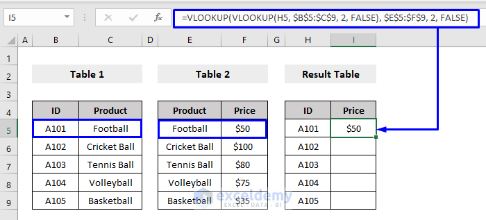
You will get the Price ($50) of ID A101 in the result cell (I5).
- Drag the row down by the Fill Handle to apply the formula to the rest of the rows and get the Prices of all the product IDs in the Result Table.
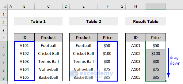
Look at the above picture, we got the Price of all the product IDs in the Result Table by running a Nested VLOOKUP formula.
Formula Breakdown:
- VLOOKUP(H5, $B$5:$C$9, 2, 0)
- Output: “Football”
- Explanation: H5 = A101, search in the data range $B$5:$C$9, that is in column index 2 (B Column), with the help of FALSE to get an exact match of the Product name “Football”.
- VLOOKUP(VLOOKUP(H5, $B$5:$C$9,2,0), $E$5:$F$9, 2, 0) -> becomes
- VLOOKUP(“Football”, $E$5:$F$9, 2, 0)
- Output: $50
- Explanation: “Football”, search in the data range $E$5:$F$9, to get an exact match (FALSE) of the Price, $50.
Method 2 – Applying Nested VLOOKUP to Get Sales Value
Steps:
- Click on the cell that you want the Sales value of the Product (e.g. cell beside Product Football in the Result Table, J5)
- Write the following formula,
=VLOOKUP(VLOOKUP(I5,$B$5:$C$9,2,0),$E$5:$G$9,2,0)I5 = Football, the Product name that we stored in the Result Table as the lookup value
$B$5:$C$9 = Data range in Table 1 to search the lookup value
$E$5:$G$9 = Data range in Table 2 to search the lookup value
2 = Column index number to search the lookup value
0 = As we want an exact match, we put the argument as 0 or FALSE.
- Press Ctrl + Shift + Enter on your keyboard.
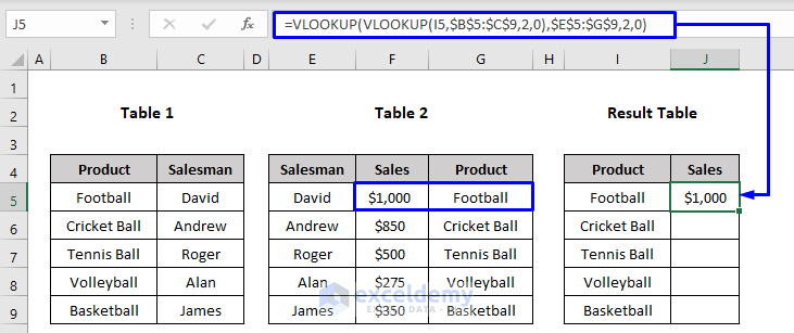
You will get the Sales value ($1,000) of Football in the result cell (J5).
- Drag the row down by Fill Handle to apply the formula to the rest of the rows to get the Sales value of all the Products in the Result Table.
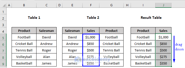
Look at the above picture, we got the Sales value of all the Products in the Result Table by running a Nested VLOOKUP formula.
Formula Breakdown:
- VLOOKUP(I5, $B$5:$C$9, 2, 0)
- Output: “David”
- Explanation: I5 = Football, search in the data range $B$5:$C$9, that is in column index 2 (B Column), with the help of 0 to get an exact match of the Salesman name “David”.
- VLOOKUP(VLOOKUP(I5, $B$5:$C$9, 2, 0), $E$5:$G$9, 2, 0) -> becomes
- VLOOKUP(“David”, $E$5:$G$9, 2, 0)
- Output: $1,000
- Explanation: “David”, search in the data range $E$5:$G$9, to get an exact match (0) of the Sales value $1,000.
Method 3 – Combining Nested VLOOKUP and IFERROR Function in Excel
In this section, we will see how to combine Nested VLOOKUP and IFERROR functions to extract a certain result from multiple tables based on one single lookup value.
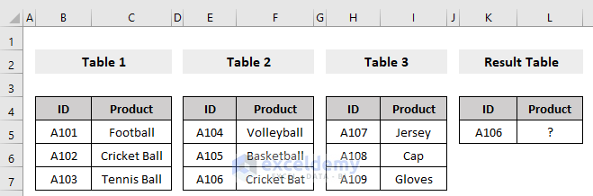
Look at the following dataset where Products are distributed in 3 different tables. We will search for a specific Product based on the ID (A106) among those 3 tables and display the result in the Product column of the Result Table.
Steps:
- Click on the cell that you want the Product name (e.g. cell beside ID A106 in the Result Table, L5)
- Write the following formula,
=IFERROR(VLOOKUP(K5,$B$5:$C$7,2,0),IFERROR(VLOOKUP(K5,$E$5:$F$7,2,0),VLOOKUP(K5,$H$5:$I$7,2,0)))Here,
K5 = A106, the ID that we stored in the Result Table as the lookup value
$B$5:$C$7 = Data range in Table 1 to search the lookup value
$E$5:$F$7 = Data range in Table 2 to search the lookup value
$H$5:$I$7 = Data range in Table 3 to search the lookup value
2 = Column index number to search the lookup value
0 = As we want an exact match, we put the argument as 0 or FALSE.
- Press Ctrl + Shift + Enter on your keyboard.
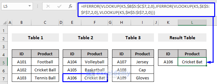
You will get the Product name (Cricket Bat) of lookup ID A106 in the result cell (L5).
Formula Breakdown:
- VLOOKUP(K5, $H$5:$I$7, 2, 0)
- Output: #N/A
- Explanation: K5 = A106, in the data range $H$5:$I$7 to get an exact match (2) of the product ID A106. As there is no match of the ID A106 in the range $H$5:$I$7 (Table 3), it returns the #N/A error.
- VLOOKUP(K5, $E$5:$F$7, 2, 0)
- Output: “Cricket Bat”
- Explanation: K5 = A106, search in the data range $E$5:$F$7 with the help of 2 (FALSE) to get an exact match of the product ID A106. We found the match of ID A106 in that range (Table 2), so it returns the “Cricket Bat”.
- IFERROR(VLOOKUP(K5, $E$5:$F$7, 2, 0),VLOOKUP(K5, $H$5:$I$7, 2, 0) -> becomes
- IFERROR(“Cricket Bat”, #N/A)
- Output: “Cricket Bat”
- Explanation: The IFERROR function checks the formula, and if it gets an error as a result, it returns another specified value by the user.
- VLOOKUP(K5, $B$5:$C$7, 2, 0)
- Output: #N/A
- Explanation: K5 = A106, search in the data range $B$5:$C$7 to get an exact match (2) of the product ID A106. As there is no match of the ID A106 in the range $B$5:$C$7 (Table 1), it returns the #N/A error.
- IFERROR(VLOOKUP(K5,B5:C7,2,0),IFERROR(VLOOKUP(K5,E5:F7,2,0),VLOOKUP(K5,H5:I7,2,0))) -> becomes
- IFERROR(#N/A, “Cricket Bat”)
- Output: “Cricket Bat”
- Explanation: The IFERROR function checks the formula, and if it gets an error as a result, it returns another specified value by the user.
Keep in Mind
- As the range of the data table array to search for the value is fixed, don’t forget to put the dollar ($) sign in front of the cell reference number of the array table.
- When working with array values, don’t forget to press Ctrl + Shift + Enter on your keyboard while extracting results. Pressing Enter will work only when you are using Microsoft 365.
Download Practice Workbook
You can download the free practice Excel workbook from here.
Related Articles
- Combining SUMPRODUCT and VLOOKUP Functions in Excel
- How to Use VLOOKUP with COUNTIF
- How to Combine SUMIF and VLOOKUP in Excel
- Use VLOOKUP to Sum Multiple Rows in Excel
- INDEX MATCH vs VLOOKUP Function
- Excel LOOKUP vs VLOOKUP
- XLOOKUP vs VLOOKUP in Excel
- How to Use IF ISNA Function with VLOOKUP in Excel
- How to VLOOKUP and SUM Across Multiple Sheets in Excel
- How to Use IFERROR with VLOOKUP in Excel
- VLOOKUP with IF Condition in Excel
<< Go Back to Advanced VLOOKUP | Excel VLOOKUP Function | Excel Functions | Learn Excel
Get FREE Advanced Excel Exercises with Solutions!
