Introduction to the Excel VLOOKUP Function
The VLOOKUP function is a powerful tool in Excel that allows you to search for a value in the leftmost column of a table and retrieve a value in the same row from a specified column. Here’s the syntax for the function:
-
Syntax
=VLOOKUP(lookup_value,table_array,column_index_num,[range_lookup])
-
Arguments
lookup_value: [required] The value you want to look up in the first column of a table.
table_array: [required] The range/table from where the function looks for the lookup value.
column_index_num: [required] This is the column index in the table from where to retrieve a value.
range_lookup: [optional] TRUE = approximate match i.e. if an exact match is not found, the function will return the closest match. FALSE = exact match.
Read More: 10 Best Practices with VLOOKUP in Excel
Method 1 – Apply Two VLOOKUP Functions Simultaneously (Nested VLOOKUP)
In this method, we use two VLOOKUP functions simultaneously, which can be more efficient than using them separately. For instance, let’s consider a dataset comprising tables of patient records at a hospital. Initially, we utilize the first VLOOKUP to search for the Serial Number of a patient, aiming to find their corresponding ID. Following this, we employ another VLOOKUP to retrieve the Patient’s Name using the ID obtained from the initial VLOOKUP. Let’s go through the steps:
Steps:
- Enter the following formula in Cell C5:
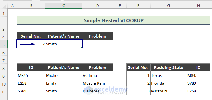
=VLOOKUP(VLOOKUP(B5,F9:H11,3,FALSE),B9:D11,2,FALSE)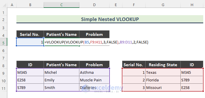
- This formula will retrieve the Patient’s Name based on a particular ID.
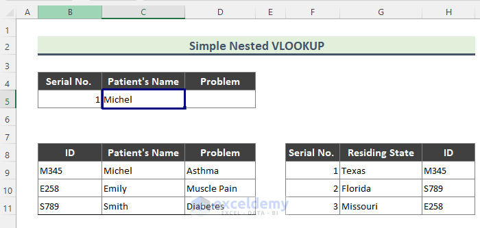
- This formula will work for any ID in the table. If you change the ID, the Patient’s Name or any other details, will change accordingly.
Breakdown of the Formula
➤ (VLOOKUP(B5,F9:H11,3,FALSE)
- The first VLOOKUP function looks for the Serial No of a patient and returns the corresponding ID from the table F9:H11.
➤ VLOOKUP(VLOOKUP(B5,F9:H11,3,FALSE),B9:D11,2,FALSE)
- The second VLOOKUP function then looks for the ID in the table B9:D11 and returns the Patient’s Name associated with that ID.
Read More: 7 Practical Examples of VLOOKUP Function in Excel
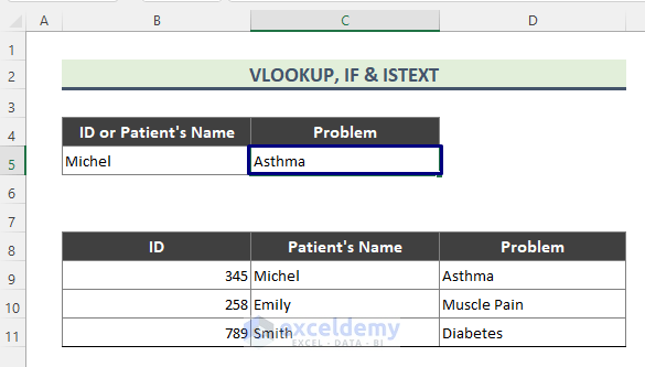
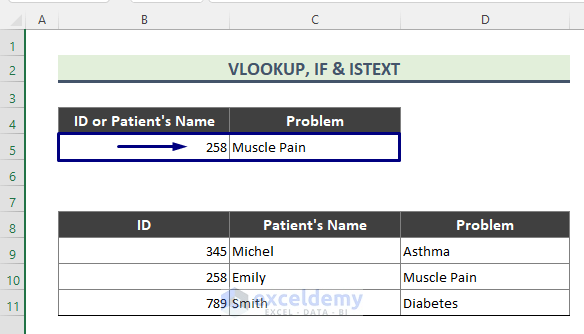
Method 2 – Double VLOOKUP with Excel IF and ISTEXT Functions
Here, we combine the IF function with two VLOOKUP functions and the ISTEXT function. Let’s discuss the steps involved:
Steps:
- Enter the following formula in Cell C5:
=IF(ISTEXT(B5),VLOOKUP(B5,C9:D11,2,FALSE),VLOOKUP(B5,B9:D11,3,FALSE))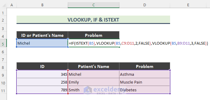
- This formula will return this result based on whether the value of B5 is text.
- If the value of B5 is not text, the following will be the result.
Breakdown of the Formula
➤ ISTEXT(B5)
- The ISTEXT function checks if the value of B5 is text or not and replies TRUE or FALSE accordingly.
➤ VLOOKUP(B5,C9:D11,2,FALSE)
- If B5 is text, the first VLOOKUP function retrieves the patient’s Problem from the range C9:D11.
➤ VLOOKUP(B5,B9:D11,3,FALSE)
- If B5 is not text, the second VLOOKUP function retrieves the patient’s Problem from the range B9:D11.
➤ IF(ISTEXT(B5),VLOOKUP(B5,C9:D11,2,FALSE),VLOOKUP(B5,B9:D11,3,FALSE))
- The IF function combines the formula and returns the result depending on the changed value of Cell B5.
Read More: How to Use VLOOKUP with Two Lookup Values in Excel
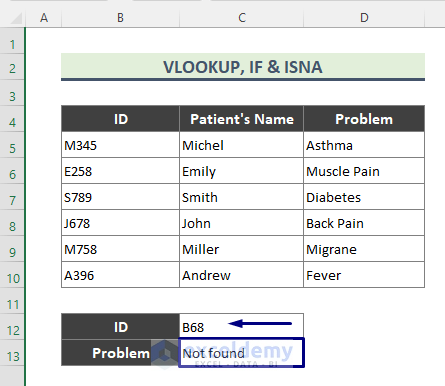
Method 3 – Double VLOOKUP with IF and ISNA Functions
In this method, we use two VLOOKUP functions with the ISNA function and the IF function. Let’s go through the steps:
Steps:
- Enter the following formula in Cell C13:
=IF(ISNA(VLOOKUP(C12,B5:D10,3,FALSE)), "Not found",VLOOKUP(C12,B5:D10,3,FALSE))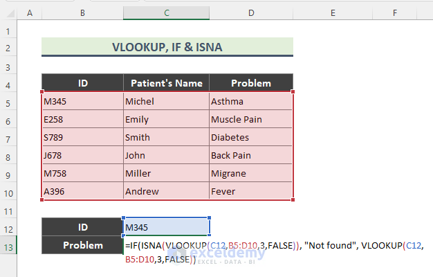
- This formula will return the result based on whether the ID is present in the specified range (B5:D10) or not.
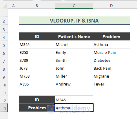
- If the ID is not present in the specified range Not Found will be returned.
Breakdown of the Formula
➤ VLOOKUP(C12,B5:D10,3,FALSE)
- The VLOOKUP function looks for the ID in the range B5:D10.
➤ ISNA(VLOOKUP(C12,B5:D10,3,FALSE))
- The ISNA function checks if the VLOOKUP result is #N/A (i.e., if the ID is not found), and returns TRUE or FALSE.
- In this table, this formula looks for M345 in the range B5:D10 and returns {FALSE}
➤ IF(ISNA(VLOOKUP(C12,B5:D10,3,FALSE)), “Not found”, VLOOKUP(C12,B5:D10,3,FALSE))
- The IF function returns Not found if the ID is not present; otherwise, it returns the patient’s Problem.
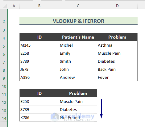
Method 4 – Double VLOOKUP with the IFERROR Function
Here, we use the IFERROR function with two VLOOKUP functions. Let’s discuss the steps involved:
Steps:
- Enter the following formula in Cell C12:
=IFERROR(VLOOKUP(B12,B5:D9,3,FALSE),IFERROR(VLOOKUP(B12,C5:D9,2,FALSE),"Not Found"))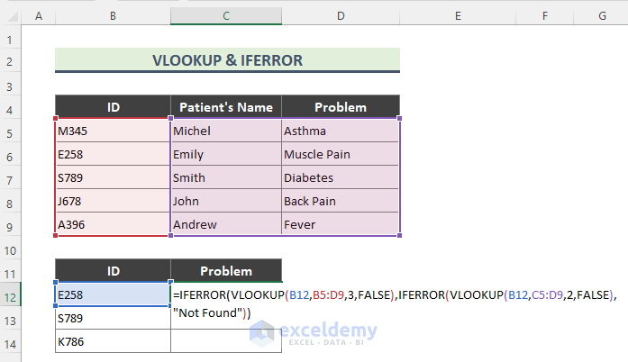
- This formula will return the result based on whether the ID is found in the specified ranges.
- Use the Fill Handle (+) to copy the formula to the rest of the cells.
Breakdown of the Formula
➤ (VLOOKUP(B12,B5:D9,3,FALSE)
- The first VLOOKUP function looks for the ID in the range B5:D9.
➤ (VLOOKUP(B12,C5:D9,2,FALSE)
- The second VLOOKUP function looks for the ID in the range C5:D9.
➤ IFERROR(VLOOKUP(B12,C5:D9,2,FALSE),”Not Found”))
- The double VLOOKUP functions wrapped with double IFERROR find the value in the dataset, and return Muscle Pain for ID: E258, otherwise, the formula returns Not Found.
Download the Practice Workbook
You can download the practice workbook from here:
Related Articles
- How to Use VLOOKUP Function with Exact Match in Excel
- How to Find Second Match with VLOOKUP in Excel
- VLOOKUP and Return All Matches in Excel
- VLOOKUP Fuzzy Match in Excel
- Excel VLOOKUP to Find Last Value in Column
- How to Use VLOOKUP to Search Text in Excel
- How to Apply VLOOKUP by Date in Excel
- Return the Highest Value Using VLOOKUP Function in Excel
- VLOOKUP with Numbers in Excel
<< Go Back to Advanced VLOOKUP | Excel VLOOKUP Function | Excel Functions | Learn Excel
Get FREE Advanced Excel Exercises with Solutions!
