VLOOKUP with Numbers in Excel (4 Examples)

The VLOOKUP function is generally used to look for a value in the leftmost column in a table and the function will return a value in the same row from the specified column. In this article, you will learn how you can use this VLOOKUP function to look up numbers under different criteria with appropriate illustrations.

VLOOKUP with Numbers in Excel: 2 Examples

1. Basic Example of Applying VLOOKUP Function with Numbers

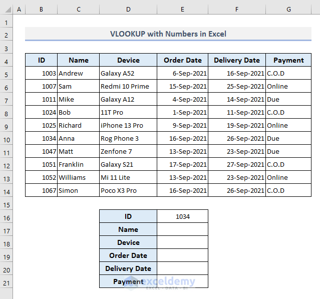
In the following table in the picture, several data containing the order details of different smartphone products have been recorded. In the output table at the bottom, we have to extract all data available from the table based on an order ID.

📌 Step 1:

➤ Select the first output Cell E17 and type the following formula with the VLOOKUP function:

=VLOOKUP($E$16,$B$5:$G$14,MATCH(D17,$B$4:$G$4,0),FALSE)

➤ Now press Enter and you’ll find the name of the customer whose order ID is 1034.

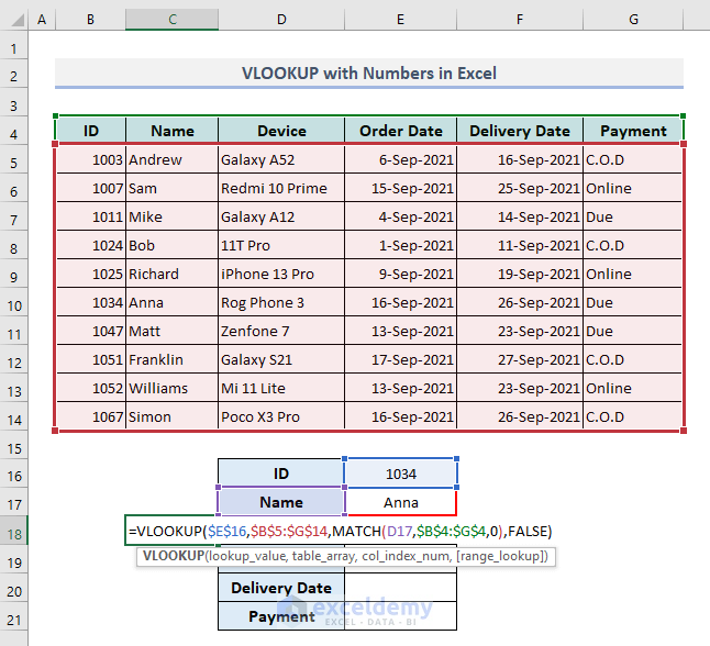
In this formula, the MATCH function has been used to define the column number of the VLOOKUP function for a particular output type.

📌 Step 2:

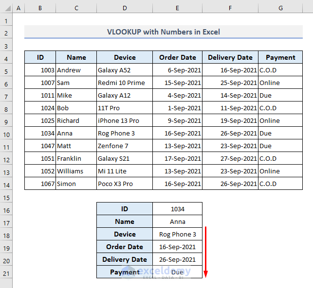
➤ Use Fill Handle now to autofill the other cells ranging from E18 to E21.

And you’ll get all available data from the table based on the specified order ID at once.

2. VLOOKUP with Numbers Formatted As Text in Excel

i. Use of Text to Columns Command

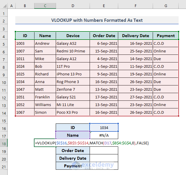
Sometimes our data table may contain numbers in text format. In that case, the previously used formula won’t work out and it will return a #N/A error as shown in the picture below. So, here we have to change the format of the ID numbers present in Column B.

📌 Step 1:

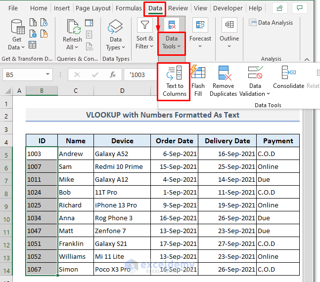
➤ Select the range of cells B5:B14 containing the order IDs first.

➤ Under the Data ribbon, select the Text to Columns command from the Data Tools drop-down.

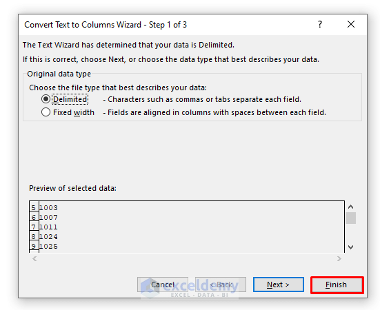
A wizard box will open up.

📌 Step 2:

➤ In the dialogue box, select the data type as delimited.

➤ Press Finish and you’re done.

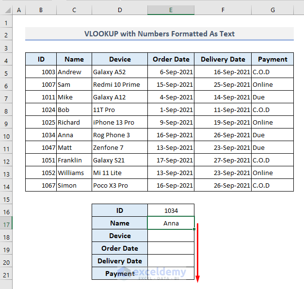
The delimiters found with the numbers will be removed now and you’ll find your IDs in number format. The previously used formula in the first output Cell E17 will now show the actual data based on the selected ID.

📌 Step 3:

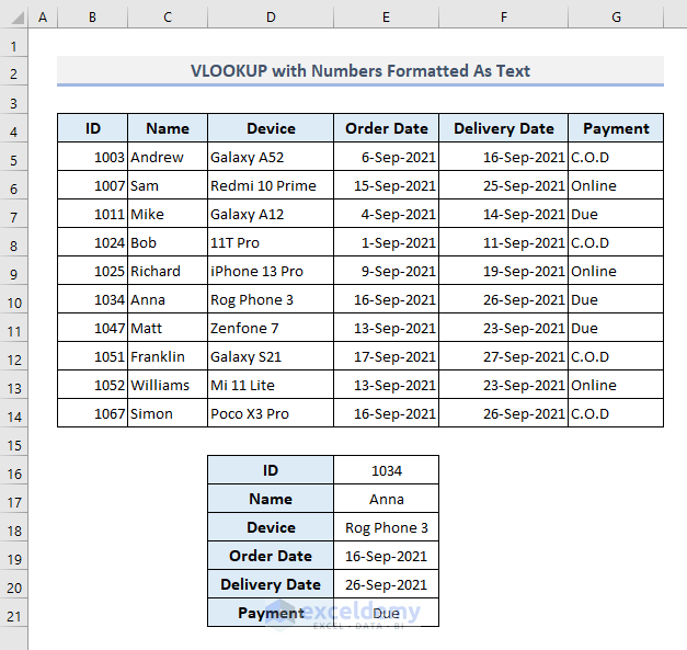
➤ Now autofill the other output cells (E18:E21) like before to get all other available data for that selected order ID.

Eventually, you’ll find all the expected data as shown in the screenshot below.

ii. Use of TEXT function with VLOOKUP

We have another option to look up an order ID in the range of cells formatted as text. We have to use the TEXT function to define the lookup_value argument in the VLOOKUP function. Thus the selected order ID number will be converted into the text format and then we’ll use this text formatted lookup value to find its duplicate in Column B.

So, the required formula in the output Cell E17 will be:

=VLOOKUP(TEXT($E$16,0),$B$5:$G$14,MATCH(D17,$B$4:$G$4,0),FALSE)

After pressing Enter and auto-filling the rest of the output cells, you’ll get all available data for the selected order ID right away.

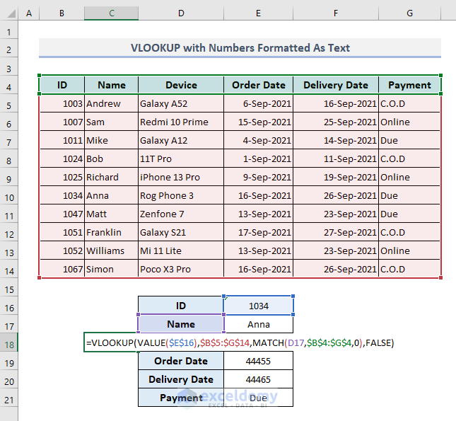
iii. Use of VALUE Function with VLOOKUP

In the last section, let’s think of an opposite case where the lookup value is in text format but the order IDs in the table are in number format. Now, we have to use the VALUE function to convert the lookup value from the text format into a number format.

In the following table, the lookup order ID in Cell E16 is in text format. So, in the first output Cell E17, while applying the VALUE function to define the lookup value, the VLOOKUP function will look like this:

=VLOOKUP(VALUE($E$16),$B$5:$G$14,MATCH(D17,$B$4:$G$4,0),FALSE)

After pressing Enter and auto-filling the rest of the output cells like before, you’ll find all the return values right away.

Download Practice Workbook

You can download the Excel workbook that we’ve used to prepare this article.

VLOOKUP with Numbers.xlsx

Concluding Words

I hope all the examples under the different criteria described above will now help you to apply them in your Excel spreadsheets while using the VLOOKUP function with numbers. If you have any questions or feedback, please let me know in the comment section.