How to Use VLOOKUP for Rows in Excel (With Alternatives)

Method 1 – Use the MATCH function to Define a Column Number from Rows in VLOOKUP

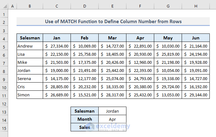
In the following picture, a dataset is presented with the amounts of sales of several salespersons over consecutive six months in a year. We’ll use the VLOOKUP function here to extract the sales value of a salesman in a specified month. We can use the MATCH function to define the column number for the specified month in E14 from the month headers.

In the output Cell E15, the required formula will be:

=VLOOKUP(E13,B5:H11,MATCH(E14,B4:H4,0),FALSE)

Press Enter and you’ll get the sales value of Jordan in April at once.

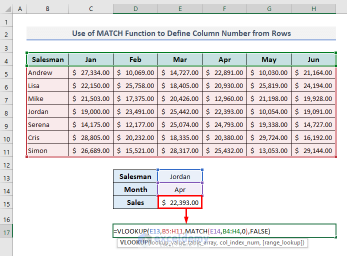
The MATCH function defines the column number for the VLOOKUP function. The VLOOKUP function then uses this column number to extract data based on the specified month from the month headers.

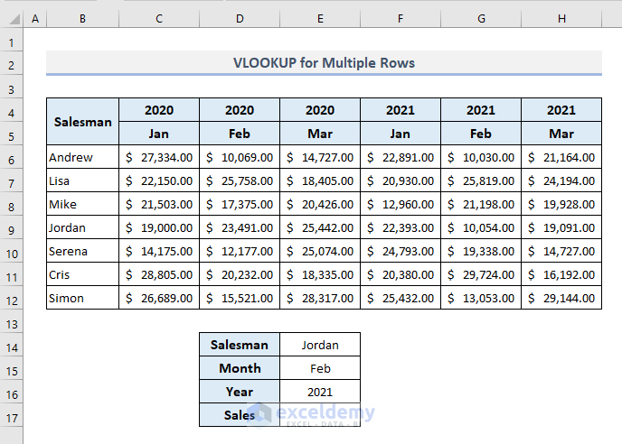
Method 2 – Use Multiple Rows with the VLOOKUP Function in Excel

Let’s use the comparative sales values over three fixed months in two different years. We’re going to extract the sales value of Jordan in the month of February 2021, which are values in E14, E15, and E16.

The required formula in cell E17 will be:

=VLOOKUP(E14,B6:H12,MATCH(E16&E15,C4:H4&C5:H5,0)+1,FALSE)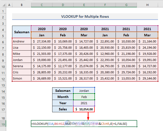

How Does the Formula Work?

The use of Ampersand (&) joins the selected month and year from the Cells E15 and E16.
The lookup array in the MATCH function has been defined by an array of pairs containing all years and months joined by the Ampersand (&).
In the lookup array of the MATCH function, the two ranges of cells have been selected starting from Column C. So, by adding ‘1’ to the MATCH function in the third argument of the VLOOKUP function, the formula will consider the index of the return column number based on the entire array of B6:H12.

Method 3 – Combining VLOOKUP with the Column Function to Return an Entire Row

Let’s use the starting dataset and fetch the sales values of a specified salesperson in C13 for all months available in the dataset.

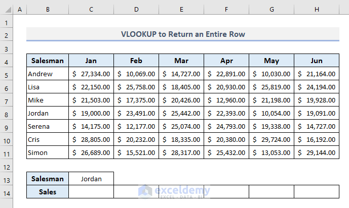
Steps:

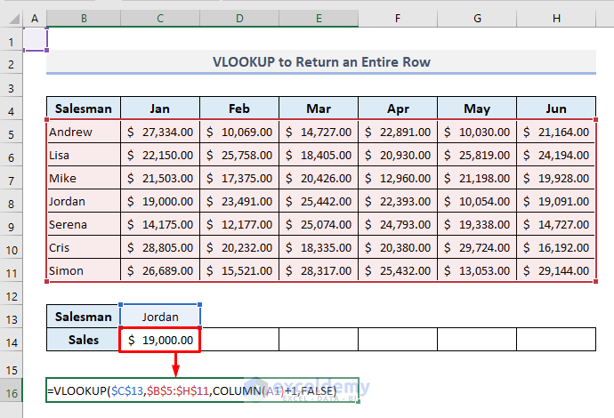
Select the output cell C14 and insert the following formula:

=VLOOKUP($C$13,$B$5:$H$11,COLUMN(A1)+1,FALSE)

Press Enter and you’ll get the sales value for Jordan in January.

Use the Fill Handle from cell C14 to autofill Row 14.

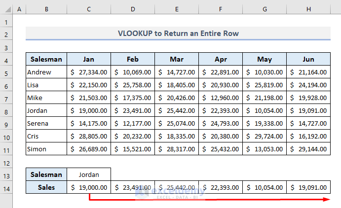
The COLUMN function has been used to alter the column numbers serially in the third argument of the VLOOKUP function while autofilling the 14th row.

Method 4 – Including an Array Formula in VLOOKUP to Extract Rows in Excel

If you want to get all the sales data for a salesperson with a single formula, use an array formula in C14 to define the column numbers in the VLOOKUP function:

=VLOOKUP(C13,B5:H11,{2,3,4,5,6,7},FALSE)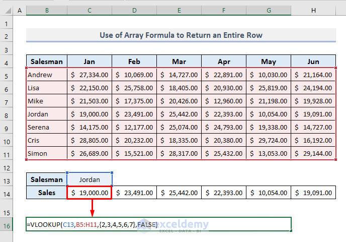

The column numbers have been defined with an array containing the index numbers of the return columns: {2,3,4,5,6,7}. The VLOOKUP function returns the outputs from these specified columns for the specified salesperson.

Two Alternatives to the VLOOKUP While Looking for Rows

Alternative 1 – Use the HLOOKUP Function to Look for Rows in Excel

The HLOOKUP function looks for a value in the top row of a table or array of values and returns the value in the same column from the specified row. The generic formula of the HLOOKUP function is:

=HLOOKLUP(lookup_value, table_array, row_index_num, [range_lookup])

Since we’re looking for the sales value of Jordan in the month of April, the required formula in Cell E15 will be:

=HLOOKUP(E14,B4:H11,MATCH(E13,B4:B11,0),FALSE)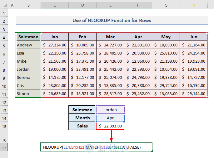

The MATCH function defines the row number of the specified salesperson in Column B.

Alternative 2 – Use the INDEX-MATCH Formula to Lookup Along Columns and Rows

The generic formula of this INDEX function is:

=INDEX(array, row_numer, [column_numer])

=INDEX(reference, row_num, [column_num], [area_num])

We can specify the row and column numbers of the INDEX function for a particular salesman in a particular month to extract the corresponding sales value.

The required formula in the output Cell E15 will be:

=INDEX(B5:H11,MATCH(E13,B5:B11,0),MATCH(E14,B4:H4,0))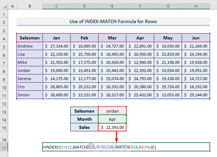

Download the Practice Workbook

VLOOKUP for Rows.xlsx