The VLOOKUP function is a game-changer when you have to retrieve information from a range of data in the same or different worksheets. This function is one of the most popular Excel functions. You can look up data, return them in a new worksheet, and sort them in ascending order. Today in this article, we will discuss three different methods to Use the VLOOKUP Ascending Order in Excel.
Overview of VLOOKUP Function in Excel
In plain language, the VLOOKUP function takes the user’s input, looks up it in the Excel worksheet, and returns an equivalent value related to the same input. This function is available in all versions of Excel from Excel 2007.
- Summary
The VLOOKUP function takes the input value, searches it in the worksheets, and returns the value matching the input.
- Syntax
- Argument
| Argument | Required/Optional | Explanation |
|---|---|---|
| lookup_value | Required | The value we want to find by searching it in another worksheet |
| table_array | Required | The range of cells in another worksheet containing out input data |
| col_index_num | Required | The specific column number in the sheet_range containing the information we want to achieve |
| [range_lookup] | Optional | The value is either TRUE or FALSE. False for an exact match and TRUE for an appropriate match. |
- Output
Returns an exact or approximate value equivalent to the user’s input value.
VLOOKUP in Ascending Order: 3 Approaches
We can return our values from the data table in the same or different worksheets and sort them in ascending order in a new worksheet. We will discuss three distinctive ways to do it.
1. VLOOKUP in Ascending Order in Same Worksheet
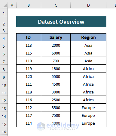
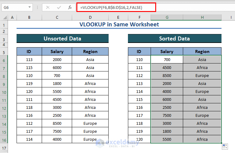
The following example includes a range of data where “ID”, “Salary”, and “Region” of some Sales Reps are given. We need to sort them in ascending order using the VLOOKUP function.
🔗 Steps:
- First, make another data table in the same worksheet where you want to retrieve the data in ascending order.
- Then, copy the ID column> Paste in the new table> go to Home tab> Sort & Filter under Editing group and select Sort Smallest to Largest as shown in the image below.
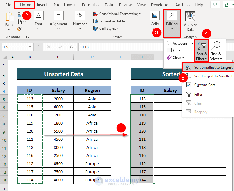
- Now, click Sort on the Sort Warning dialog box.

- Now, the values of the ID column will be sorted in ascending order.
- Next, apply the VLOOKUP function in the “Salary” column.
The final form of this formula is:
=VLOOKUP(F6,B$6:D$16,2,FALSE)Where,
- Lookup_value cell is F6
- Table_array is B$6:D$16
- Col_index_num is 2
- [range_lookup]: we want the exact match (FALSE).
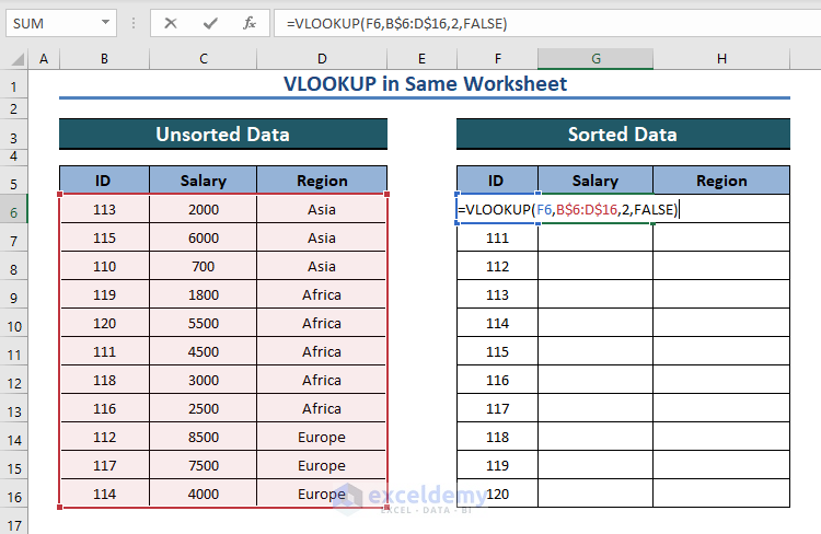
- Then, press ENTER to get the result.
- Now, drag the Fill Handle tool downward to Autofill the formula to the next cells.

- Hence, we get the Salary for the corresponding ID no.
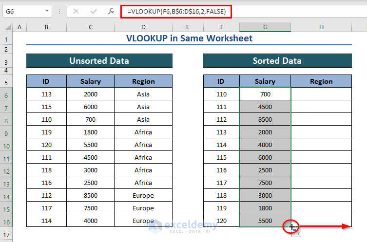
It is noticeable that we have used the lookup range as “B$6:D$16” which means we have locked the column. So with copying or dragging the formula, the cell reference won’t change itself further. If we had used Absolute cell reference (i.e. $B$6:$D$16), both the row and column would have been frozen. Read this article to copy formulas without changing cell reference and this one for changing one reference only.
- After that, drag the mouse to the right end to get the same result in the remaining cells.
Read More: How to Use VLOOKUP for Multiple Columns in Excel
2. VLOOKUP in Ascending Order from Another Worksheet
In this section, we will perform the same task again for looking up another sheet.
🔗 Steps:
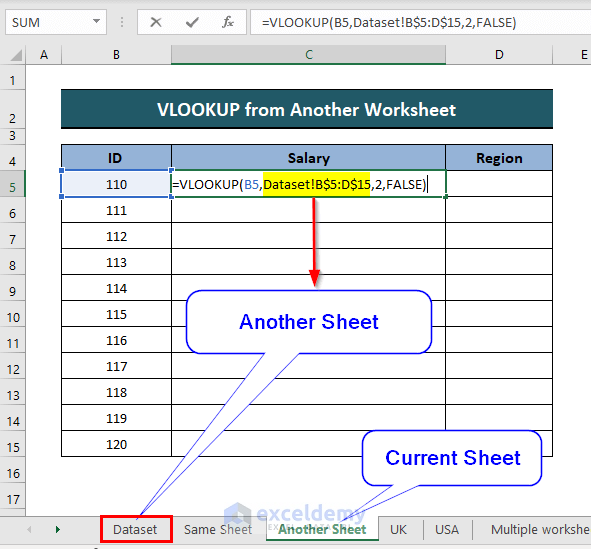
- First, create a data table in another worksheet where you want to return data in ascending order according to your lookup value.
- Then, copy all the data from the ID column and sort them following this step of Method 1.

- Next, apply the formula below to lookup values from a different sheet.
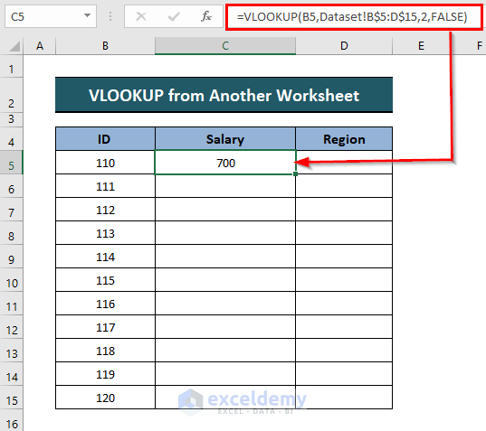
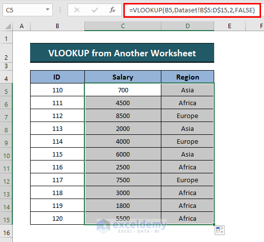
=VLOOKUP(B5,Dataset!B$5:D$15,2,FALSE)
Where,
- Lookup_value is B5
- Table_array is Dataset!B$5:D$15. Click on the Dataset sheet and select the cell range B5:D15
- Col_index_num is 2
- [range_lookup]: we want the exact match (FALSE).
- Now, press ENTER to get the result.
- Finally, repeat these steps of Method 1 to fill the other blank cells with the same formula.
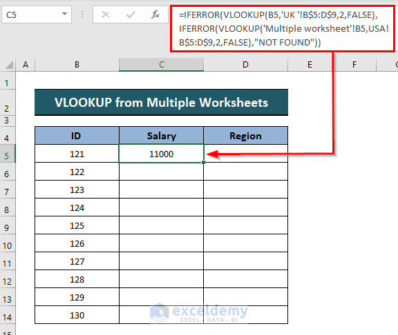
3. From Multiple Worksheets with IFERROR
We can look up our data in multiple worksheets and then sort them in ascending order by using the VLOOKUP with the IFERROR function.
We have two data worksheets in which we will look up the value. One of them got data for “UK”.

And the other worksheet contains data for the “USA”.

This method will look up for value in every worksheet until it finds the exact value that we are looking for.
🔗 Steps:
- Firstly, create a new data workspace in a new worksheet where we want to sort our data in ascending order. Copy all the data from the ID column and sort them following this step of Method 1.

- Now, apply the “VLOOKUP” along with the “IFERROR” function combinedly.
The format for this formula is:
So, the final look of the formula is:
=IFERROR(VLOOKUP(B5,'UK '!B$5:D$9,2,FALSE),IFERROR(VLOOKUP('Multiple worksheet'!B5,USA!B$5:D$9,2,FALSE),"NOT FOUND"))
- After that, press ENTER and repeat these steps of Method 1 to fill the other blank cells with the same formula.
- Finally, we have got our values in ascending order.

Read More: How to Use VLOOKUP to Return Multiple Columns in Excel
Common Problem for VLOOKUP Ascending Order
Using the “VLOOKUP” function in ascending order is comparatively easy. However, you might face problems while ascending in order using this function if you don’t use the fourth argument of this function. Let’s discuss.
VLOOKUP Ascending Order Without Exact Match
There is an optional argument in the VLOOKUP function that plays a vital role when we sort in ascending order. That argument is the 4th argument (range_lookup). Let’s see how this argument works.
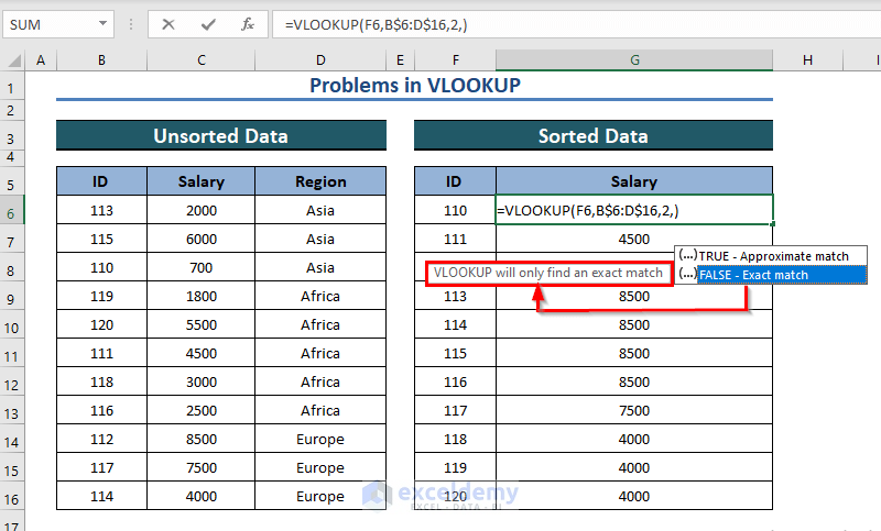
- In the following example, we will find the Salary from the ID in ascending order.
- Here, apply the “VLOOKUP” function in cell “G6”.
=VLOOKUP(F6,B$6:D$16,2)
In the formula,
- Lookup_value is F6
- Table_array is B$6:D$16
- Col_index_num is 2
We will ignore the range_lookup. The “VLOOKUP” function will then automatically select the range_lookup as “Approximate match (TRUE)”.

- Now, press ENTER to get the result.

From the result, we can see that we did not get the result in ascending order. Because, when the 4th argument is TRUE or omitted, you will get an unexpected result. Then the function will look for an approximate match which you may not want for the lookup value in ascending order. Therefore we get this unexpected result. From the picture, we can see we got a Salary “8500” for ID “112-116” and “4000” for ID “118-120”.
Solution for VLOOKUP Ascending Order Without Exact Match
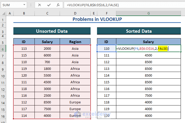
We can solve this problem just by applying the argument in the function correctly.
Edit the applied VLOOKUP function. In the function argument, we see the 4th argument. Now we will use this.
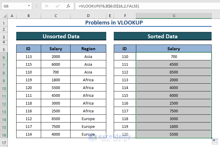
Select “FALSE” as your 4th argument to get the “EXACT” match for your lookup value. This time we will retrieve our values in ascending order.
Now, press ENTER. The problem is solved and we got our values in ascending order.
Things to Remember
➤ The VLOOKUP function always searches for lookup values from the leftmost top column to the right. This function “Never” searches for the data on the left.
➤ If there is a multiple highest value in a worksheet, the “VLOOKUP” will only return the first match in the list.
➤ Always use the 4th argument as “FALSE” to get the exact result.
➤ The “VLOOKUP” function is not “case-sensitive”. It does not process upper and lower case text differently.
Conclusion
Lookup for data in ascending order using the VLOOKUP function is discussed in this article. Though this function is difficult for the new users to comprehend, we tried to make it as simple as possible. Hope this article is useful to you when you are facing problems. You are welcome to share your thoughts if you have any confusion.
Further Readings
- VLOOKUP from Multiple Columns with Only One Return in Excel
- How to Use VLOOKUP Function to Compare Two Lists in Excel
- VLOOKUP with Drop Down List in Excel
- How to Use VLOOKUP for Rows in Excel
- How to Use Column Index Number Effectively in Excel VLOOKUP
- Perform VLOOKUP by Using Column Index Number from Another Sheet
- How to Find Column Index Number in Excel VLOOKUP
<< Go Back to Issues with VLOOKUP | Excel VLOOKUP Function | Excel Functions | Learn Excel
Get FREE Advanced Excel Exercises with Solutions!
