Step 1: Creating a Data Table
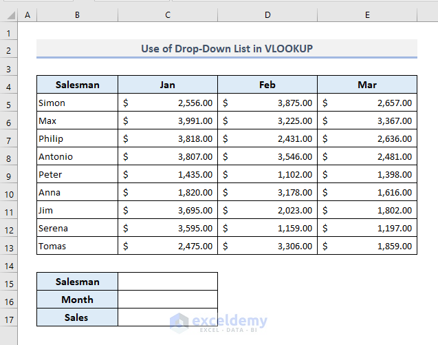
To use the VLOOKUP function with the drop-down lists, we need a dataset. The following picture shows a random dataset, with the sales amounts for some salespersons recorded based on months.
There’s another table at the bottom where the salesman and month names must be chosen from the drop-down lists. So, in C15 and C16 cells, we must assign the drop-down criteria for salesmen and months.
In the output Cell C17, we’ll insert the VLOOKUP function to extract the sales for a particular salesman in a particular month.
Step 2: Defining the Range of Cells with a Name
Steps:
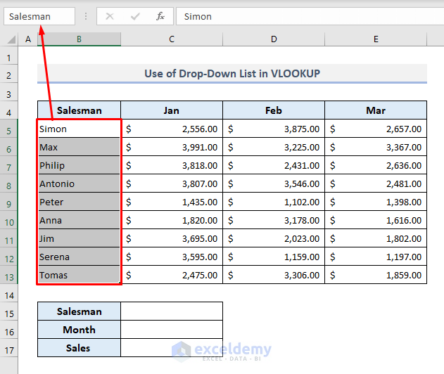
- Select the range of cells B5:B13.
- In the Name Box, situated at the top-left corner, give a name to the selected range of cells. In our example, we defined the range of cells by the name ‘Salesman’.
Step 3: Setting Up the Drop Down Lists
Steps:
- Select Cell C15.
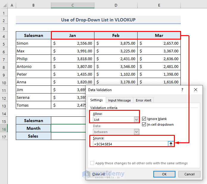
- Choose the Data Validation command from the Data Tools drop-down under the Data tab.
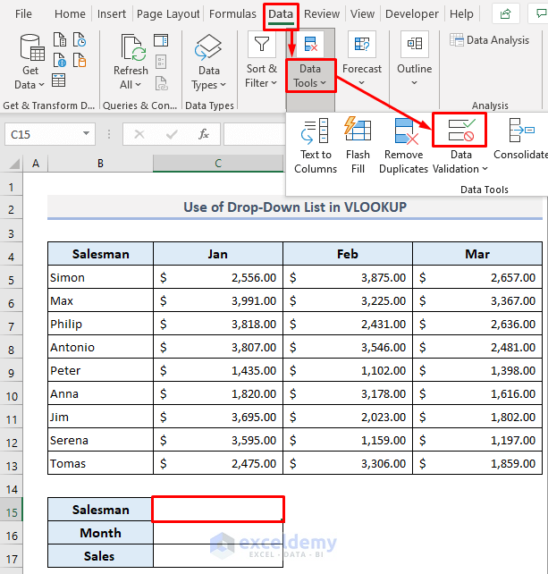
You’ll find a dialogue box named Data Validation.
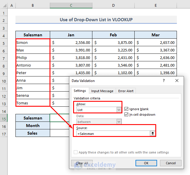
- In the Allow box, select the List option.
- In the Source box, type:
=Salesman
- Or, select the range of cells B5:B13.
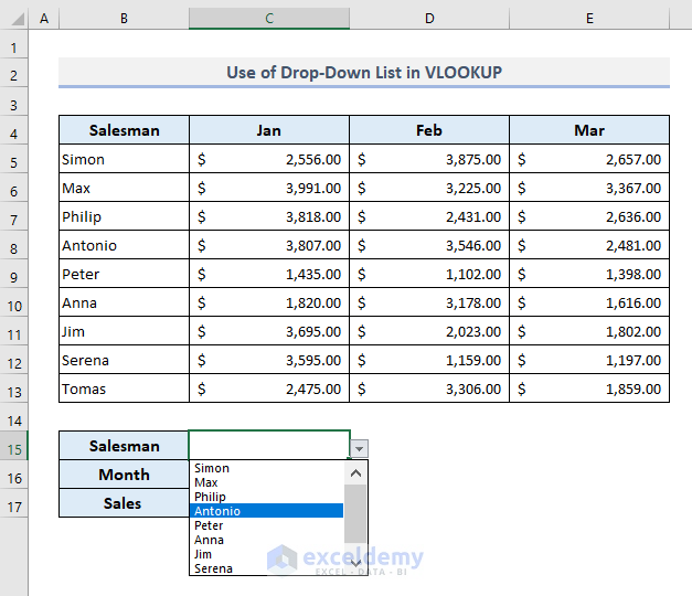
- Press OK, and you’ll have just made the first drop-down list for the salesmen.
You have to create another drop-down list for the months.
- Select Cell C16 and reopen the Data Validation dialogue box.
- In the Allow box, choose the List option.
- In the Source box, select the range of cells (C4:E4) containing month names.
- Press OK.
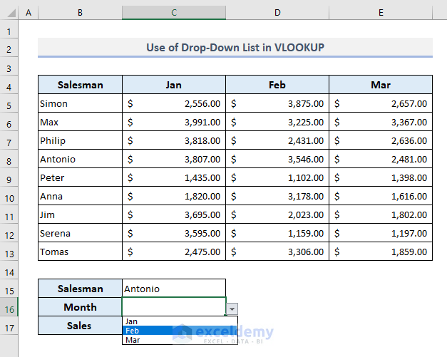
Both drop-downs are now ready to display the assigned values.
Step 4: Using VLOOKUP with Drop-Down Items
Steps:
- Select the name of a salesman from the drop-down list in C15.
- Select the month name from the drop-down in C16.
- In the output Cell C17, enter the following formula:
=VLOOKUP(C15,B5:E13,MATCH(C16,B4:E4,0),FALSE)- Press Enter and you’ll find the sales value of Antonio for the month of February at once.
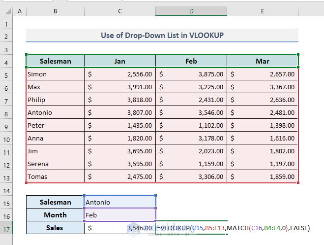
In this formula, the MATCH function has been used to define the column number of the selected month.
Download the Practice Workbook
You can download the Excel workbook to practice.
Related Articles
- How to Use VLOOKUP for Multiple Columns in Excel
- VLOOKUP from Multiple Columns with Only One Return in Excel
- How to Use VLOOKUP to Return Multiple Columns in Excel
- How to Use VLOOKUP Function to Compare Two Lists in Excel
- How to Use the VLOOKUP Ascending Order in Excel
- How to Use VLOOKUP for Rows in Excel
- How to Use Column Index Number Effectively in Excel VLOOKUP
- Perform VLOOKUP by Using Column Index Number from Another Sheet
- How to Find Column Index Number in Excel VLOOKUP
<< Go Back to Advanced VLOOKUP | Excel VLOOKUP Function | Excel Functions | Learn Excel
Get FREE Advanced Excel Exercises with Solutions!
