Method 1 – Using VLOOKUP with Array Formula
- Suppose you have a dataset with smartphone models and their specifications.
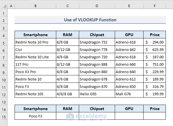
- To extract all specifications for a specified smartphone (e.g., Poco F3), enter this array formula in cell C15:
=VLOOKUP(B15,B5:F12,{2,3,4,5},FALSE)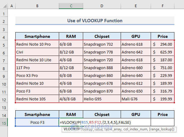
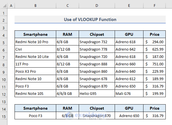
- Press Enter to retrieve all specifications at once.
Read More: 10 Best Practices with VLOOKUP in Excel
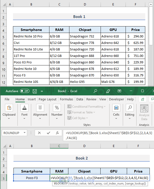
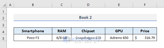
Method 2 – Applying VLOOKUP to Return Multiple Columns from a Different Workbook
- Assume you have a primary data table in an Excel workbook named Book 1.
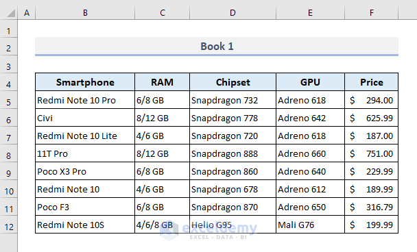
- In another workbook (Book 2), enter this formula in cell C5 to extract specifications from Book 1:
=VLOOKUP(B5,'[Book 1.xlsx]Sheet1'!$B$5:$F$12,{2,3,4,5},FALSE)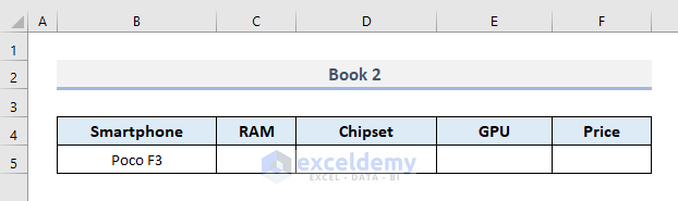
- Keep Book 1 open to avoid a #N/A error.
Press Enter and you’ll get the specifications for the selected device.
Read More: 7 Practical Examples of VLOOKUP Function in Excel
Method 3 – Inserting VLOOKUP to Sum Return Values from Multiple Columns
- Suppose you have sales data for different salesmen over 5 days.
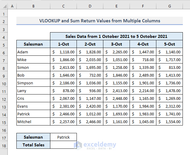
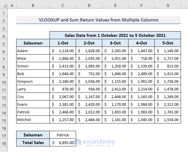
- To find the total sales for a specific salesman (e.g., Patrick), enter this formula in cell C18:
=SUM(VLOOKUP(C17,B6:G15,{2,3,4,5,6},FALSE))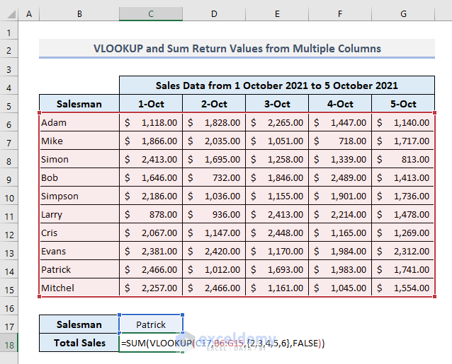
- Press Enter to get the total sales amount.
Method 4 – Combining VLOOKUP with COLUMN Function
- Extract specifications for Poco F3 without an array formula by entering the following formula in Cell C15:
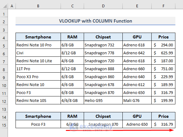
=VLOOKUP($B$15,$B$5:$F$12,COLUMN(C$4)-1,FALSE)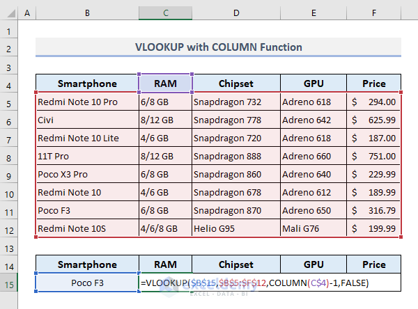
- Press Enter and drag the Fill Handle rightward to autofill for other devices.
An Alternative to the VLOOKUP to Return Multiple Columns in Excel
Consider using the INDEX and MATCH functions as an alternative to VLOOKUP for returning multiple columns. The formula in cell C15 would be:
=INDEX(B5:F12,MATCH(B15,B5:B12,0),{2,3,4,5})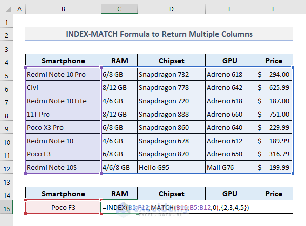
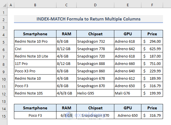
- Press Enter.
- This retrieves specifications from multiple columns for the selected smartphone device.
Download Practice Workbook
You can download the practice workbook from here:
Related Articles
- How to Use VLOOKUP for Multiple Columns in Excel
- VLOOKUP from Multiple Columns with Only One Return in Excel
- How to Use VLOOKUP Function to Compare Two Lists in Excel
- How to Use the VLOOKUP Ascending Order in Excel
- VLOOKUP with Drop Down List in Excel
- How to Use VLOOKUP for Rows in Excel
- How to Use Column Index Number Effectively in Excel VLOOKUP
- Perform VLOOKUP by Using Column Index Number from Another Sheet
- How to Find Column Index Number in Excel VLOOKUP
<< Go Back to Advanced VLOOKUP | Excel VLOOKUP Function | Excel Functions | Learn Excel
Get FREE Advanced Excel Exercises with Solutions!
