VLOOKUP and Return All Matches in Excel (7 Ways)

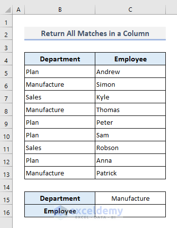
Method 1 – VLOOKUP and Return Multiple Matches in a Column

We have a table containing random names of several employees and their departments. We want to show the names of the employees in a single column who are working in the manufacturing department. If you’re an Excel 365 user, you can go for the FILTER function.

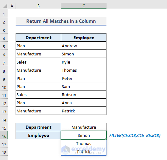
• With the FILTER function, the required formula in the output Cell C16 will be:

• Hit Enter.

• If you’re using an older version of Microsoft Excel, use the following combined formula:

• Hit Enter.

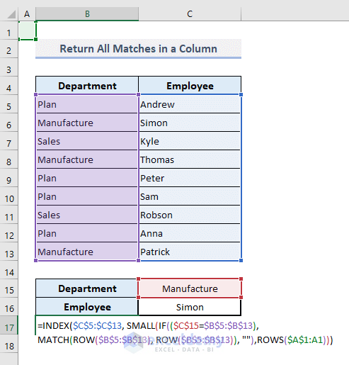
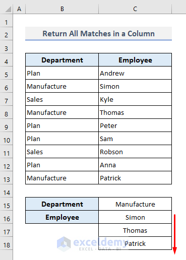
• By dragging the Fill Handle from Cell C16 down, you’ll get the rest of the names of the employees from the specified department.

How Does This Formula Work?

• ROW($B$5:$B$13): The ROW function extracts the row numbers of the defined cell references and returns the following array:

{5;6;7;8;9;10;11;12;13}

• MATCH(ROW($B$5:$B$13), ROW($B$5:$B$13)): The MATCH function here converts the extracted row numbers starting from 1. So, this part of the formula returns an array of:

{1;2;3;4;5;6;7;8;9}

• IF(($C$15=$B$5:$B$13), MATCH(ROW($B$5:$B$13), ROW($B$5:$B$13)), “”): With the help of the IF function, this part of the formula returns the index number of the rows that meet the specified condition. So, this part returns an array of:

{“”;2;””;4;””;””;””;””;9}

• The SMALL function in the formula pulls out the first small number found in the previous step and assigns this number to the second argument (row_number) of the INDEX function.
• Finally, the INDEX function shows the name of the employee based on the specified row number.
• The ROWS function in this formula defines the k-th number for the SMALL function. While using Fill Handle to fill down the rest of the cells, the formula uses this k-th number to extract data followed by the SMALL function.

Read More: How to Use VLOOKUP Function with Exact Match in Excel

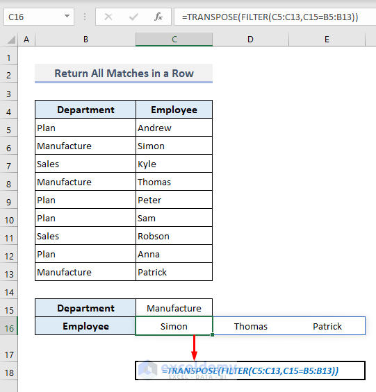
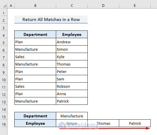
Method 2 – VLOOKUP and Return All Matches in a Row in Excel

• If you’re using Excel 365, insert the following function:

• Press Enter and you’ll be shown the names of the employees from the Manufacture department in a horizontal array.

• If you don’t use Excel 365, use the following function:

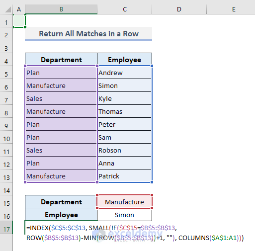
• Drag the Fill Handle down until you find the first #NUM error.

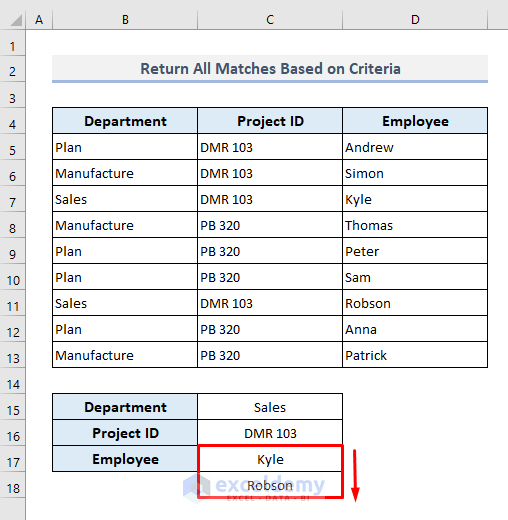
Method 3 – VLOOKUP to Return Multiple Values Based on Criteria

We’ve added an extra column in the middle of the table. This column stores the project IDs that are assigned to the corresponding employees present in Column D. We want to know the names of the employees who are currently working in the Sales department on the project ID of DMR 103.

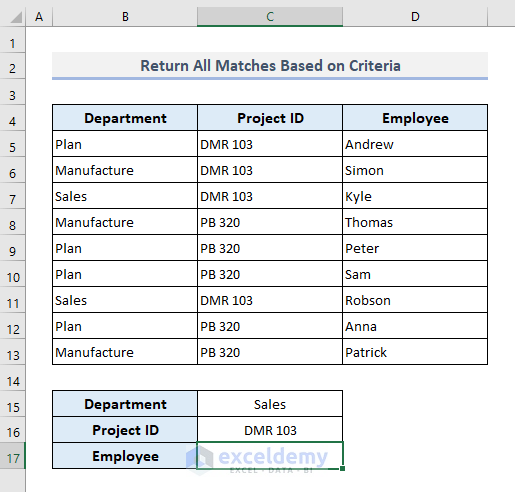
• The required formula in the output Cell C17 will be:

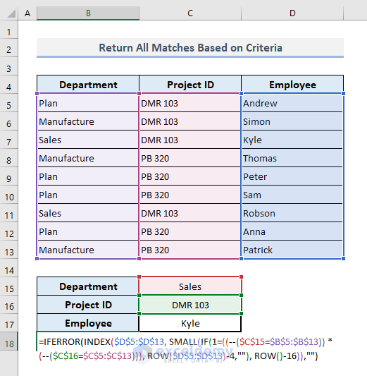
• Fill down Cell C17 to show the rest of the names with the given conditions.

Some Important Features of this Formula:

• The IFERROR function has been used to show a customized output if any error is found.
• The IF function in this formula combines two different criteria and with the help of double-negative, the boolean values (TRUE or FALSE) turn into 1 or 0. The function then returns the index number of the rows that have matched with the given criteria.
• ROW($D$5:$D$13)-4: In this part, the number ‘4’ is the row number of the Employee header.
• ROW()-16: The numerical value ‘16’ used in this part denotes the previous row number of the first output cell.

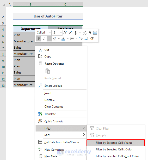
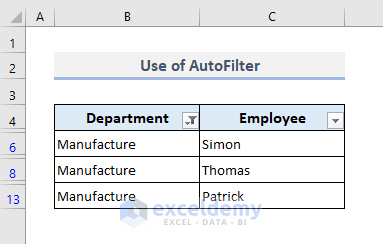
Method 4 – VLOOKUP and Draw Out All Matches with AutoFilter

Steps:

• Select the entire data table and right-click the mouse.
• Choose the Filter by Selected Cell’s Value option from the Filter options.

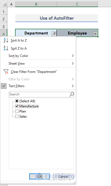
• Click on the Filter button from the Department header.
• Check the Manufacture option only.
• Press OK.

• You’ll be displayed the filtered data.

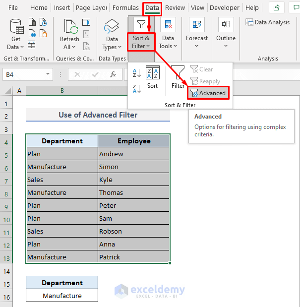
Method 5 – VLOOKUP to Extract All Matches with the Advanced Filter in Excel

Steps:

• Select the entire data table.
• Under the Data tab, click on the Advanced command from the Sort and Filter drop-down.
• A dialog box named Advanced Filter will open up.

• Select the entire data table for the List Range input.
• Choose B15:B16 for the input of the Criteria Range.
• Press OK.

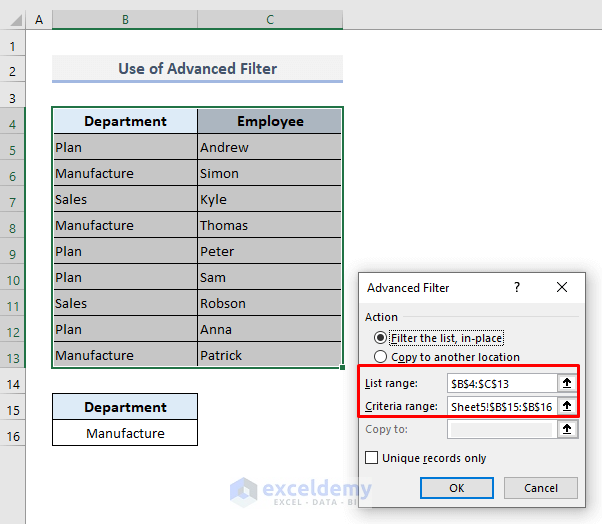
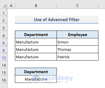
• You’ll be displayed the filtered result with the names of the employees from the Manufacture department only.

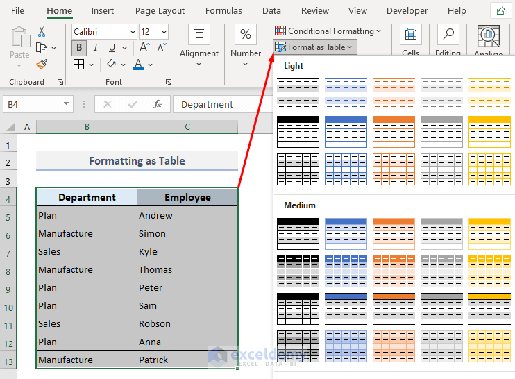
Method 6 – VLOOKUP and Return All Values by Formatting as Table=

Steps:

• Select the entire dataset.
• From the Format as Table drop-down under the Home tab, choose any of the tables you prefer.

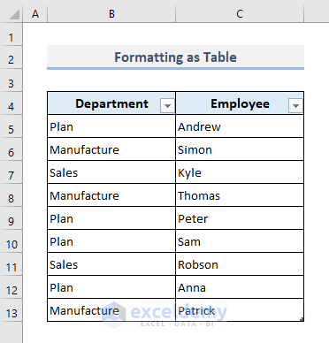
• Here’s the sample table.

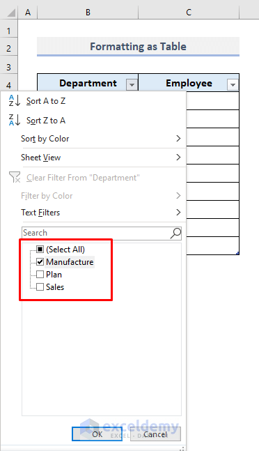
• Select the Manufacture option after clicking on the filter button from the Department header.
• Press OK.

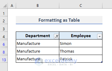
• The screenshot below shows the outputs based on the specified selection.

Method 7 – VLOOKUP to Pull Out All Matches into a Single Cell in Excel

• The required formula in the output Cell C16 will be:

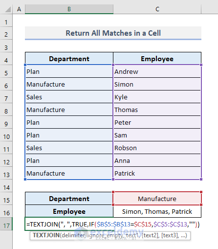
Read More: How to Use VLOOKUP to Search Text in Excel

Download the Practice Workbook

Related Articles

• How to Use VLOOKUP with Two Lookup Values in Excel
• How to Apply Double VLOOKUP in Excel
• How to Find Second Match with VLOOKUP in Excel
• VLOOKUP Fuzzy Match in Excel
• Excel VLOOKUP to Find Last Value in Column
• How to Apply VLOOKUP by Date in Excel
• Return the Highest Value Using VLOOKUP Function in Excel
• VLOOKUP with Numbers in Excel

<< Go Back to Advanced VLOOKUP | Excel VLOOKUP Function | Excel Functions | Learn Excel