How to Use VLOOKUP for Multiple Columns in Excel?

Method 1 – Getting Values from Multiple Columns Using Excel VLOOKUP Function

Consider the following starting dataset, containing Product Details for some products, which will be used to demonstrate VLOOKUP functionalities in multiple columns.

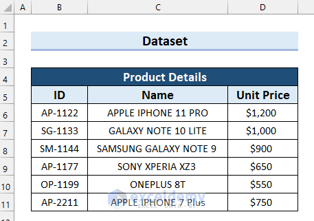
With the starting dataset, the results will be used for another table: Sales Overview, with ID, Name, Unit Price, Quantity, and Total Sales. The goal is to automatically calculate the Total sales in the table by entering just the product ID. The formula will extract product names and prices from the Product Details table via VLOOKUP.

Steps:

Select the cell where you want the product Name, cell C15.
Use the following formula in the cell:

=VLOOKUP(B15,$B$6:$D$11,{2,3},0)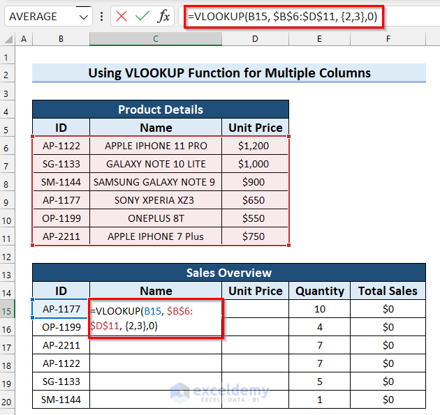

Press Enter to apply the formula. If you are using a version older than Excel 2019, press Ctrl + Shift + Enter.

How Does the Formula Work?

In the VLOOKUP function, the first argument is carrying the data which will be searched in the table. Here B15 contains the ID which is going to be matched with the product list table ID.
$B$6:$D$11 is the table array range where the data will be searched.
{2,3} means the function is extracting the second and third column values of the matched rows.
0 is defining that you need an exact match.

Drag the Fill Handle down to copy the formula to the other cells in the column.

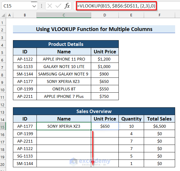
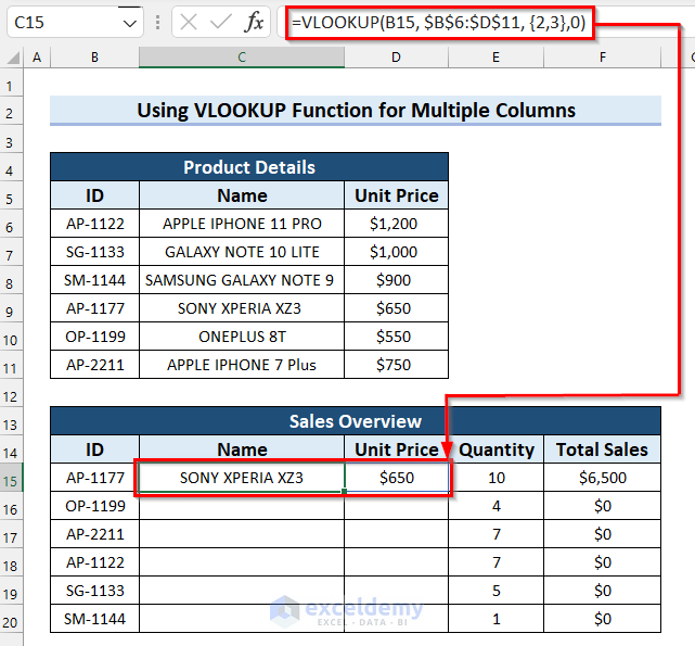
Here’s how the output should look for the last cell.

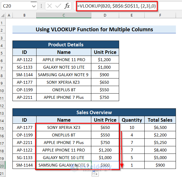
Generating the total sales for F15 uses a simple multiplication:

=D15*E15

Which is then copied in the column to F20.

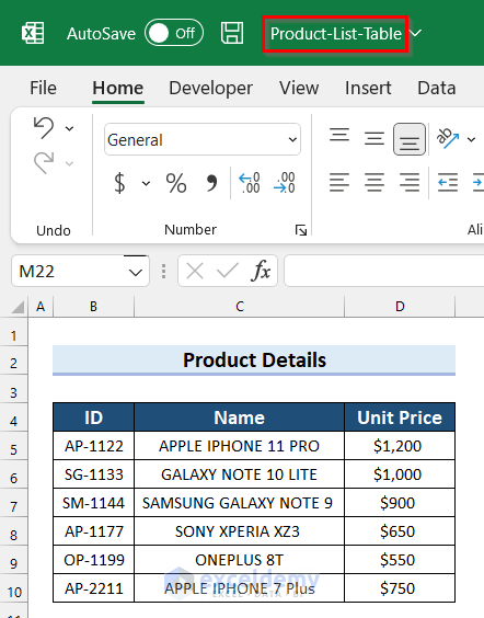
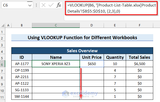
Method 2 – Using the VLOOKUP Function for Multiple Columns from Different Workbooks

Unlike in the previous method, the two tables will be located in different workbooks (files) in the same folder.

Steps:

Select the cell where you want the product Name (C6 in the example).
Copy the following formula into the selected cell. Note that the formula uses the exact name of the source Excel workbook so you’ll need to change it accordingly.

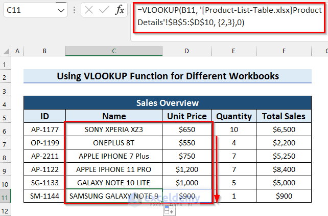
=VLOOKUP(B6,'[Product-List-Table.xlsx]Product Details'!$B$5:$D$10,{2,3},0)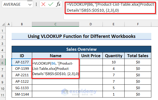

Press Enter to get the result. For Excel versions older than Excel 2019, use Ctrl + Shift + Enter.

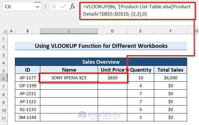
The function is the same as the previous method’s formula. The only difference is that since the source table is in another file it needs to be referenced through the Workbook’s file name and sheet first: ‘[Product-List-Table.xlsx]Product Details’!

Drag the Fill Handle down to copy the formula.

After copying, the cells should automatically populate with values.

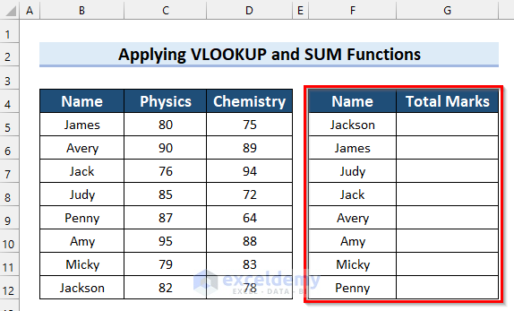
Method 3 – Applying VLOOKUP to Find Values from Multiple Columns in Excel

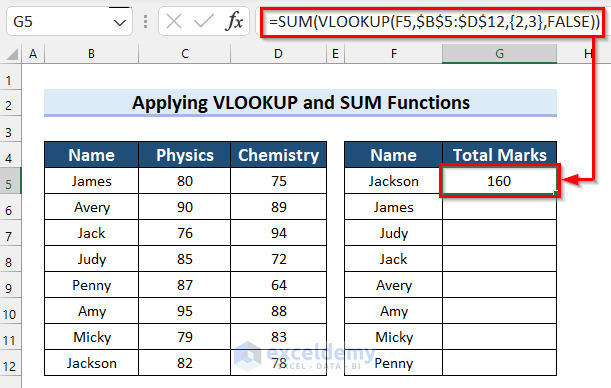
Suppose you have the Name of some students and their obtained marks in Physics and Chemistry, such as in the example table below. You have another table that has the names only and you want to show the total marks beside their name. You can use VLOOKUP to fetch and perform other functions with those values.

Steps:

In Cell G5, the first cell you need the results for, copy the following formula:

=SUM(VLOOKUP(F5,$B$5:$D$12,{2,3},FALSE))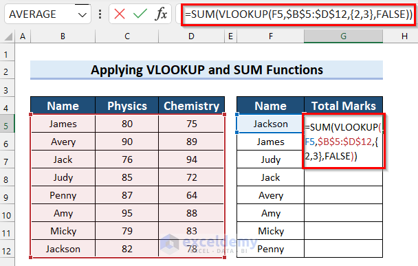

Press Enter to apply it. If you are using a version of Excel older than 2019, you will need to press Ctrl + Shift + Enter.

How Does the Formula Work?

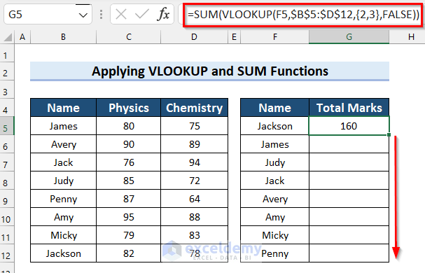
VLOOKUP(F5,$B$5:$D$12,{2,3},FALSE): Here, in the VLOOKUP function, F5 is the lookup_value, $B$5:$D$12 is the table_array, {2,3} as col_index_num, and FALSE as range_lookup. The formula returns the matches for the lookup_value from columns 2 and 3 of the table_array.
SUM(VLOOKUP(F5,$B$5:$D$12,{2,3},FALSE)): Now, the SUM function returns the sum of the two values it got from the VLOOKUP function.

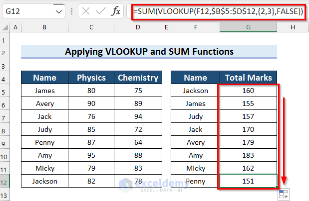
Drag the Fill Handle down to copy the formula to the other cells.

Here’s how the results should look in the sample table after the cells have been filled.

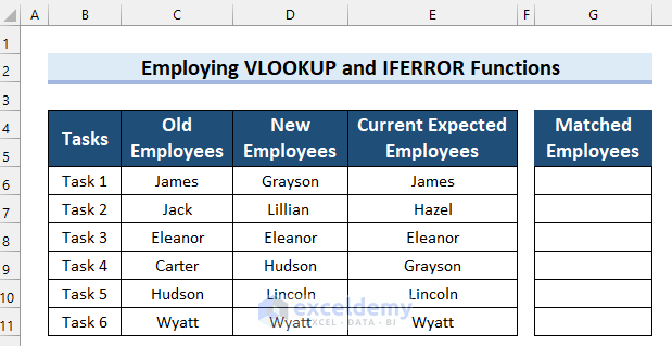
Method 4 – Combining Excel VLOOKUP and IFERROR Functions to Compare Multiple Columns

For this section, consider a dataset of Tasks and the names of employees who were assigned to them. There is a column that contains the names of Old Employees who were assigned to that task, the names of New Employees who were assigned to that task, and the names of Current Expected Employees for those tasks. Here’s how you can see if an employee name matches across all three columns.

Steps:

Copy the following formula into G6 (the first cell in the results column):

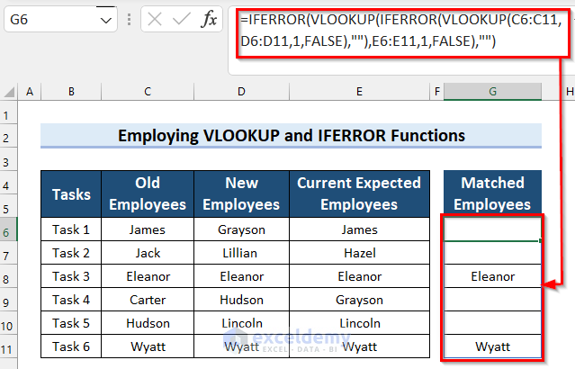
=IFERROR(VLOOKUP(IFERROR(VLOOKUP(C6:C11,D6:D11,1,FALSE),""),E6:E11,1,FALSE),"")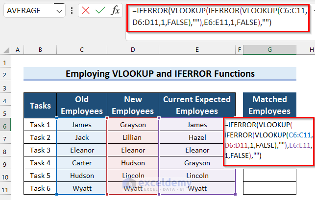

Press Enter to get the result. If you are using an older version of Microsoft Excel than Excel 2019 then press Ctrl + Shift + Enter.

How Does the Formula Work?

VLOOKUP(C6:C11,D6:D11,1,FALSE): This part of the formula compares the Old Employees column and the New Employees column.
IFERROR(VLOOKUP(C6:C11,D6:D11,1,FALSE),””): Now, the IFERROR function replaces the #N/A with an empty string.
VLOOKUP(IFERROR(VLOOKUP(C6:C11,D6:D11,1,FALSE),””),E6:E11,1,FALSE): Here, the VLOOKUP function compares the Current Expected Employees column against the matching values returned from the first VLOOKUP function.
IFERROR(VLOOKUP(IFERROR(VLOOKUP(C6:C11,D6:D11,1,FALSE),””),E6:E11,1,FALSE),””): Finally, the IFERROR function replaces the #N/A with an empty string.

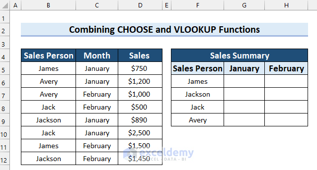
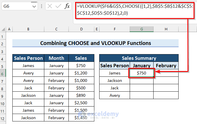
Method 5 – Joining Excel CHOOSE and VLOOKUP Functions for Multiple Criteria

Consider a dataset of sales information with Sales Person, Month, and Sales. Let’s streamline the table to show a person’s total sales across months and put the results in a new table.

Steps:

Go to Cell G6 and write the following formula:

=VLOOKUP($F6&G$5,CHOOSE({1,2},$B$5:$B$12&$C$5:$C$12,$D$5:$D$12),2,0)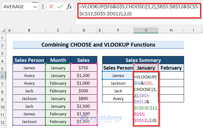

Press Enter to apply the formula. Versions of Microsoft Excel older than Excel 2019 will need Ctrl + Shift + Enter.

How Does the Formula Work?

CHOOSE({1,2},$B$5:$B$12&$C$5:$C$12,$D$5:$D$12): Here, in the CHOOSE function, I selected {1,2} as index_num, $B$5:$B$12&$C$5:$C$12 as value1, and $D$5:$D$12 as value2. This formula returns the value using the index_num.
VLOOKUP($F6&G$5,CHOOSE({1,2},$B$5:$B$12&$C$5:$C$12,$D$5:$D$12),2,0): Now, the VLOOKUP function finds the match and returns a value accordingly.

Drag the Fill Handle down to copy the formula.

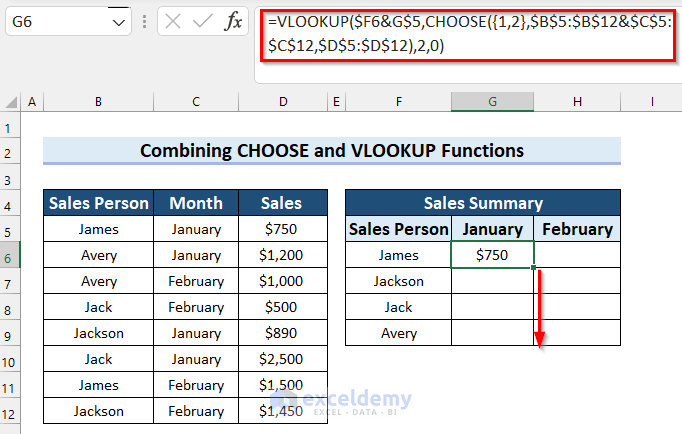
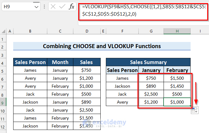
Drag the Fill Handle to the right to apply the formula to the next column.

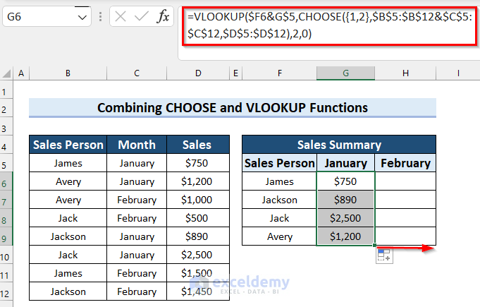
Here’s the final result:

Method 6 – Merging VLOOKUP and MATCH Functions to Lookup Value Dynamically

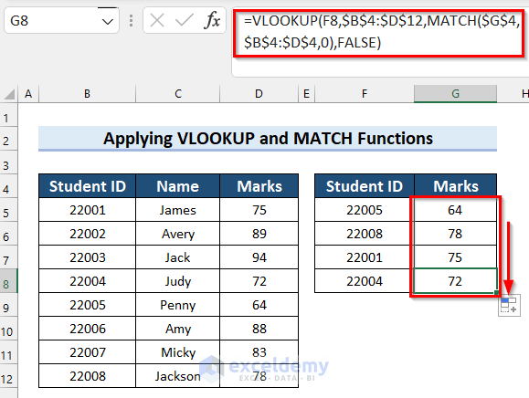
Consider the following dataset for this example, which contains the Student ID, Name, and Marks. Let’s make a formula that automatically finds the marks for a student based on their ID.

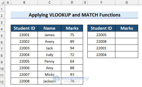
Steps:

Select cell G5 and input the following formula:

=VLOOKUP(F5,$B$4:$D$12,MATCH($G$4,$B$4:$D$4,0),FALSE)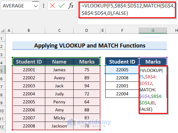

Press Enter to get the result.

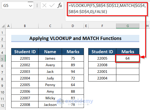
How Does the Formula Work?

MATCH($G$4,$B$4:$D$4,0): Here, in the MATCH function, I selected $G$4 as lookup_value, $B$4:$D$4 as lookup_array, and 0 as match_type. The formula will return the relative position of the lookup_value in the lookup_array.
VLOOKUP(F5,$B$4:$D$12,MATCH($G$4,$B$4:$D$4,0),FALSE): Now, the VLOOKUP function returns the match.

Drag the Fill Handle down to copy the formula.

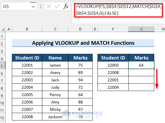
Here’s how it should look. You can replace the values in the F column and track how the results change automatically. Alternatively, you can replace “Marks” in the G header with “Name” and see that the function fetches names instead. This is due to the MATCH function matching column headers between the tables.

Alternative to VLOOKUP Function for Multiple Columns in Excel

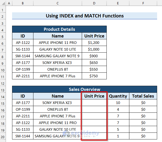
To illustrate how powerful the VLOOKUP function is, here’s what you’d need to do with the INDEX function and the MATCH function to emulate a part of it. Consider the same dataset used in the first VLOOKUP method. Let’s find the Unit Price of the product using the Name and ID.

Steps:

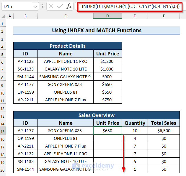
Select cell D5 and copy the following formula:

=INDEX(D:D,MATCH(1,(C:C=C15)*(B:B=B15),0))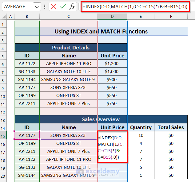

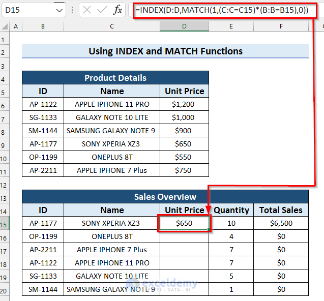
Press Enter to get the result. For Excel versions older than 2019, press Ctrl + Shift + Enter.

How Does the Formula Work?

MATCH(1,(C:C=C15)*(B:B=B15),0): This part of the formula matches the entered ID and Name with the dataset, and the “1” here refers to TRUE as in return the row number where all the criteria are TRUE.
INDEX(D:D,MATCH(1,(C:C=C15)*(B:B=B15),0)): Now, the INDEX function returns the value from the range D:D.

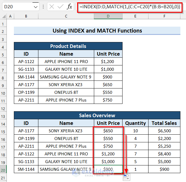
Drag the Fill Handle down to copy the formula to the other cells.

Here’s the final result:

Related Content: How to Use Dynamic VLOOKUP in Excel

Common Errors While Using These Functions

Common Errors	When They show
#N/A Error	This error will occur in older Excel versions if the formula is an array formula, and you just press Enter. To solve it, press CTRL + SHIFT + ENTER.
#N/A in VLOOKUP	The lookup value does not exist in the table. The lookup value is misspelled or contains extra space. The table range is not entered correctly. You are copying VLOOKUP, and the table reference is not locked.
#VALUE in CHOOSE	If index_num is out of range, CHOOSE will return a #VALUE error.
Range or an array constant	CHOOSE function will not retrieve values from a range or array constant.
#VALUE in INDEX	All ranges must be on one sheet otherwise INDEX returns a #VALUE error.